 |
Biology 103 Fall 2006 Laboratory Forum
|
|
Comments are posted in the order in which they are received,
with earlier postings appearing first below on this page.
To see the latest postings, click on "Go to last comment" below.
Go to last comment
Darwin's Voyage Revisited Revisited
Name: Paul Grobstein
Date: 2006-09-12 09:10:38
Link to this Comment: 20359 |
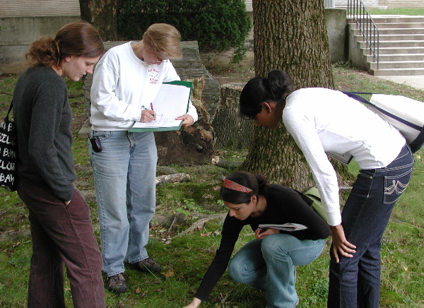
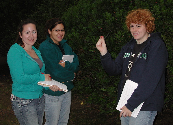
Life has recently been discovered on two planets, currently named Nearer and Farther. Survey expeditions are being undertaken to characterize life on each, with the objective of comparing the charcteristics of life on the two planets both with each other and with life on earth. The general effort is to better understand general properties of living systems.
Expeditionary groups have been formed to undertake an initial survey of "plant" life on Nearer and Farther. Plant life on earth is characterized by substantial diversity; there are a large number of different kinds of plants. The goal of the expeditionary groups is to try and determine whether diversity of plant life is an idiosyncracy of life on earth or a more general property of life wherever it is found.
You are a member of one such expeditionary group. Your group must return with a scheme for categorizing plant life on the planet assigned that is well motivated by your observations, clearly described, and yields a definite quantitative result for the numbers of kinds of plants on that planet. You will of course need to use understandings of the meaning of "plant" derived from experiences on earth, but you should not presume that categories of plant life on Nearer and Farther are necessarily similar to those on Earth. Your report should note presumptions about what plants are, be clear about what observations motivate your categorizing scheme, provide some indication of the level of confidence you have in your quantitative results, and discuss what further observations are motivated by your findings . A preliminary report of your studies will be presented at a conference on "Diversity in BioSystems: New Findings From Additional Cases", focused on the question of whether "diversity" is or is not a fundamental characteristic of living systems.
Your group should also publish a summary of its findings in this forum. Be sure to include in the text of your summary the names of all team members.
Some related readings:
documentation
Name: Paul Grobstein
Date: 2006-09-12 15:06:06
Link to this Comment: 20362 |
Expedition photgraphs are available
here. To include photos in your reports type
<img src="URL" width=200 align=right>
Use your browser to get the URL of the image you want. Use the "preview for HTML" to check that the image appears as you want it. Image size can be adjusted by varying the number following width=
Planet Nearer Research Findings
Name: Georgia, C
Date: 2006-09-12 15:22:34
Link to this Comment: 20364 |
Diversity in BioSystems: New Findings From Additional Cases
By Georgia Lawrence, Corey Norcross, Crystal Reed, and Simone Biow
After researching our collections of matter from the planet Nearer, we determined a general definition of plant life from our observations. Plant life consists of organic matter, meaning not man- made, that must be rooted in or on other organic matter in order to develop and sustain life. Plants also develop and follow some sort of life cycle.
We have chosen to classify each plant by its distance from the where it is rooted into other organic matter. While similar species may be found at differing heights, each organism is classified by the highest point at which it was observed. One organism cannot be in multiple classes, if a organism is found at a different height in later observations, its classification must be changed. Classifications are as follows:
Class 1: 0-3 inches
Class 2: 3-9 inches
Class 3: 9 inches- 5 feet
Class 4: 5- 15 feet.
Class 5: 15 feet and up.
Since we are basing our system on our observations on one particular day, and not over extended lengths of time, we felt this was the best way to classify the different plants that we found.
Qualitative Results:
Class 1: 14 plants
Class 2: 5 plants
Class 3: 1 plants
Class 4: 2 plants
Class 5: 2 plants
Total: 24 plants
As future observers continue to document plants on the planet Nearer, updates will need to be made in accordance with changes in height, and the addition of new plants found in various locations.
Name: Angely Mon
Date: 2006-09-12 15:23:20
Link to this Comment: 20365 |
Category 1 � varying shades of green, protruding from ground, long and stringy
2 different types-
1. patches of longer, stringy onion-smelling protrusions, smaller in number of patches, uniformly greener.
2. shorter, more varying colors, more common/prevalent
3. attached to some of the green stem protrusions were yellowish and purplish, delicate, soft, thin structures that easily broke apart when pulled from ground. More aesthetically pleasing to the eye than perhaps the monotony of the rest of the other green structures.
4. there were also dark green, very dense structures that covered a large portion of the ground. It seemed to tangle up in itself and grew in multiple directions from one starting point. It is made up of thin, green tear-like structures.
Category 2 � taller than us (at least 4 average-sized women tall), dark brown body structure, extends in different directions forming arm-like structures. Attached are paper-thin, small (3 inches long) with very little depth, sharper structures.
1. ones attached to the arm-like structures tend to be greener, and more vibrant looking. They are completely flat and straight across.
2. Ones on the ground are browner, drier, and more shriveled.
a. This suggests a change in temperature or weather.
b. Sun might have something to do with growth/change in these because of the differing colors/textures.
Category 3 � Dry, dark, where all the plant life originates from. Some spots are harder and bumpy, other spots are less bumpy and more flat. Gritty texture when picked up, not completely covered leaving the surface exposed. Protrusions from surface appears to be in good health perhaps indicating nutrients that are present.
1. texture- other substances have been found that contribute to the uneven feel, such as tiny pieces of rounded, hardened material
2. color- very deep, dark, brownish color; moisture in some parts affects the color to some degree (lighter or darker)
Category 4 � another form of ground protrusion but larger than the life found in category 1 but smaller than category 2. At least � of average woman tall and about 3-4 average women wide. Dark green in color, smaller extensions than category 2 with long, pointed paper-thin structures
1. roundish, reddish attachments found on the ends of the needle-like structures
2. could possibly be a source of food, similar to berries found on earth (visually).
Farther Finder's Findings
Name: Sarah G, M
Date: 2006-09-12 15:25:00
Link to this Comment: 20366 |
Team: Farther Finder
Plant(s) presumptions:
� have a base/root
� are self-reproducing
� need water
� need sunlight
� make their own food
Observations:
� Planet Farther gets lots of direct sunlight
� open to the natural environment-gets water/wind
� in a valley with trenches on the far sides
� plants are close to the ground
� different heights between ground height
� different growth rates
� has a relationship with different organisms
� DIVERSITY
Diversity
� of locations
� amount of plants
� size of the plants
� growth of the plants
Categories
A: spongy like material, close to the soil, spread out, grows horizontally, absorbs the least amount of sunlight, receives more moisture and nutrients from the soil and decomposition
B: more vertical growth in clumps and patches, tufts of varying heights, age is a factor (regarding color and size), resilient, many in competition with each other, species have some flowering and fruition
C: variety of species within the category, growth is upright and across, usually taller than those plants in category B, mainly located in the trenches that have less sunlight, adaptable to different soils, two species have a better survival rate than the others from the same category, grows flowers
D: a variety of species but they all seem to have a solid structure with a somewhat rounded shape, grows from a central location, branches are small/thin//compact, there are small fruits/nuts
E: app. three species in differing locations, it seems that size pertains to how much sunlight is received, difference density and height
Smallest plant life (E1)
� get the least amount of water but most amount of sun.
� also have a large surface area
� grows away from the center the most
Mid-sized plant life (E2)
� the ground was even, level ground
� received some sunlight
� spread of branches but less of a spread found in E1
Large sized plant life (E3)
� grows more up than out because it retains more water
� grows in trenches, on a slope
� the plants from category C surround the base root of this plant
Name:
Date: 2006-09-12 15:25:25
Link to this Comment: 20367 |
The following names are included in the previous comment:
Courtney Malpass
Melson Jones
Angely Mondestin
Karen Ginsburg
Nearer Team 2
Name: M. Hume, K
Date: 2006-09-12 15:36:21
Link to this Comment: 20368 |
Observational Table for Estumpos
Estompo 1
Roughly 1 meter in diameter, overturned on side, resembles a section of the Tronco; has similar characteristics to Tronco but has more moisture and is not connected to the ground. Between Arbol 1 and 2
Estompo 2
Roughly 1 meter in diameter, resembles a section of the Tronco; has similar characteristics to Tronco but has more moisture and is not connected to the ground. Between Arbol 1 and 2.
Estompo 3
Roughly 1 meter in diameter, resembles a section of the Tronco; has similar characteristics to Tronco but has more moisture and is not connected to the ground. Between Arbol 1 and 2
All three estompos seem to be a lifeless form resembling the Tronco estructure of Arbol 1; however, it is not connected to other parts of the Arbols, but instead divided and broken.
Arbol 1.
Estrella Verde
5 points, serrated edge, complex internal system, vibrant green On tree
Estrella Marron 5
points, serrated edge, complex internal system, dull brown, significantly smaller than E.V. On ground
Espinitas Vivas
Spiked orb, scaly center, heavy, possible fruit, green with brown edges On tree
Espinitas Muertas
Spiked orb, scaly center, lighter, possible fruit, dull brown, dessicated, smaller On ground
Tronco
Large, cylindrical structure, main body of Arbol 1 On tree
Madera
Covers Tronco, has vertical markings, overall brown with different shades, dry, rough On tree
Ramas
Extend from tree in upward curvature, various sizes On tree
Raizes
Snakelike, different widths, underground and above ground On tree
Moco
Green, moist, furry texture, grows on both bark and ground not near the dry dirt On tree
Arbol 1 is a continiously extended body in which all its components (leaves, trunk, fruit, roots, and bark) are interconnected. The moss is also found in dark, moist places but not near the area where Arbol 1 is found; it is also present in various areas around Planet Nearer, therefore it is not part of Arbol 1.
Arbol 2.
Lagrima
Teardrop shaped, complex internal system, green, serrated edge On tree
Banquitos
Grow vertically, brown in color, smoother texture than Arbol 1 On tree
Moco
Green, moist, furry texture, grows on both bark and ground not near the dry dirt On tree
Raizes
Snakelike, different widths, underground and above ground On ground
Tronco
Tall, cylindrical shaped, thinner than Arbol 1, light brown spots throughtout, body overall brown. On tree.
Madera
Thinner in width than Arbol 1, darker brown color, softer. Found on tree.
Arbol 2, like Arbol 1 is a continiously extended body in which all its components (leaves, trunk, fruit, roots, and bark) are interconnected. The moss is also found in dark, moist places but not near the area where Arbol 2 is found; it is also present in various areas around Planet Nearer, therefore it is not part of Arbol 2. Arbol 1 is the same species as Arbol 2, but it is a different kind of plant in physical characteristics.
Observations on Pasto
Similar to the structure and texture of Estrella Verde, but thinner, longer, and growing out of ground evenly, growing on entire planet except around Arbols. We believe this may be due to the competition of nutrients, as the Pasto growing around the Arbols is not as healthy looking, and lacks proper nutrients.
Name: Farther Fi
Date: 2006-09-12 15:37:37
Link to this Comment: 20369 |
members:
Sarah Gale
Moira Nadal
Ingrid Paredes
Kelly Soudachanh
Further Expedition
Name: Meagan, Ke
Date: 2006-09-13 15:04:17
Link to this Comment: 20391 |
PLANET FURTHER EXPEDITION TEAM MEMBERS: Meagan McDaniel, Masha Kapustina, Cayla McNally, Kelsey McMillen
Our findings concerning the nature of plant life on Planet Further led us to many discoveries about the diversity and nature of life in biospheres outside Planet Earth. We were struck, for example, by the obvious physical distinctions and similarities between the different species of flora on Planet Further. Lacking sufficient time to observe the full life cycles of Planet Further�s native plants, we classed our observations based on immediate physical distinctions between the species, and our native Earth presumptions of what constitutes a plant.
The following features summarize our belief of what constitutes a plant, both living and dead.
� A plant is an organism which is predominantly stationary and receives the bulk of its nutrient intake through the soil.
� A plant has an organized shape that includes visible symmetry, and definite borders.
� A plant interacts with its environment through the use and donation of energy.
� A plant goes through a life cycle that includes reproduction and death, and possesses mechanisms for self-defense.
� A plant is composed of different substances which interact within itself to perpetuate its own existence.
We sought a way to classify Planet Further�s plants into categories based on simple physical observations, owing to our lack of knowledge concerning the plants� composition, life cycle, or interactions with the environment. Total, we collected samples of thirty distinct species of plants on our expedition to Planet Further; since we could not contain the entire organism, we used samples from each that were similar in structure and can therefore be assumed to be similar in function.
CATEGORY 1. Location.
We divided up our samples based on the locations where they were collected relative to the ground, from which we assume the plants gain their nutrients.
ABOVE EYE LEVEL: 11 species
AT EYE LEVEL: 7 species
BELOW EYE LEVEL: 12 species
CATEGORY 2: Shape.
We further subdivided these samples based on their relative shape, working with the assumption that similarly-shaped species would belong to the same family.
ABOVE EYE LEVEL: 5 different shapes, including wide and round, thin and pointed, and jagged.
AT EYE LEVEL: 3 different shapes, including narrow, round, and multi-shaped.
BELOW EYE LEVEL: 3 different shapes, including long and thin, round-edged, and serrated.
Furthermore, we observed the texture of each sample and discovered that most seemed waxy in nature, though there were some samples that felt dry. One in particular displayed sharp serrated edges that we believe are used for self-defense against potential consumers. This observation, combined with samples that seemed to have been eaten at, imply the existence of additional life that consumes these plants for energy.
Name:
Date: 2006-09-13 15:07:51
Link to this Comment: 20392 |
Farther Team 2
Hannah Mueller, Kali Noble, Sarah Mellors
Observations:
� All specimens are green with leaves
� Plant height varies and is divided into three categories
� Some plants have waxy leaves others do not
� Some leaves are long and skinny (bladed) others are wide
Method of division based upon observations:
Division I: Plant Height
Short (under 1 foot): 13 specimens
Medium (1-6 feet): 2 specimens
Tall (6 feet and up): 4 specimens
Division II: Blades or Non Blades
Blade-A long narrow smooth edged leaf with parallel veins that come to a point at the tip.(5 specimens)
Non Blades- A wide potentially jagged edged leaf with webbed veins. (14 speciments)
Division III: Non Blades Leaf shape
Jagged versus Smooth edges
Jagged: (6 specimens)
Smooth: (8 specimens)
Observations about Planet Nearer
Name: Nearer Gro
Date: 2006-09-13 15:07:58
Link to this Comment: 20393 |
**Claire, Carolina, Amelia, Annabella***
In order to determine whether the objects on Planet Nearer were alive her not, we went through the following criteria for observing. They include smell, green color (contained green or the plant itself was green fully), roots, stalks, extensions, and whether when part of the plant was broken it produced a sticky greenish substance.
Our initial observations of planet Nearer lead us to believe that there were many different types of plants and vegetation present. We categorized the plants by
1.) height
2.) texture : a) bark b) roots c) leaf
3.) shape : a) bark b) roots c) leaf
4.) reproductive mechanism : a) seeds b)flower c) spores d) berrries
5.) color
MOSS:
In terms of height, the moss was closest to the ground and most horizontally oriented. Of the mosses, there were three different types: One was star-shaped, located in the dirt, and had a medium green color, the second was coral-shaped, was growing in the dirt, and had a light green color, and the third was growing on the tree, was sparser than the other two, and was olive colored.
GRASS:
Most of the grass we saw was about ankle-height, however, there were five different varieties. The first one had short and thick blades, the second had stringy long stalks with sprouts, the third had a long stem from which short stubby blades were growing. The fourth had a split blade and the leaf protruded at 90 degrees. The fifth was short, fragile, and clumped, was matte in texture and bluish color.
CLOVER:
The clovers were a little bit higher than the grass. The first variety was the tallest of the clovers, had a three-leaf shape, and a white triangle pattern on the leaves, and minty scent. The second was similar to the first in shape, except it was much smaller in height and lacked the white triangular pattern. The third was relatively short and single-leafed, with a round heart-shaped leaf.
DANDELION GREENS:
We found a variety of dandelions with four long serrated leaves. There was only one dandelion variety present.
FERNS:
The first fern was growing in close proximity to the tree, was about ankle-high, and had a longer extension of it with seeds, so we could not determine whether it was one plant variety or two different ones. It is possible that the plant changes shape and texture as it matures, however, we would need more different samples to determine the characteristics of the plants physical stages of life. The second fern had rounder leaves which grew off the stem opposite each other. The third fern had seeds at the top of the plant and round leaves.
SHRUBS:
The shrubs were all about six feet tall. We saw three shrubs, all of which had concealed roots. The first was dark green with spikey leaves, red berries, had a round shape at the top, and the branches spread out in an orderly fashion. The second one was spindly, had a variety of leaf color, thin light-colored branches, and no berries. The third had small cutaneous leaves which were a light green color, and the branches spread out in a chaotic manner.
TREES:
The tallest were the trees, of which there were two. They were about 48 feet high (about 4 stories). Both trees had branches which spread in a horizontal orientation and which had a leaves. One tree had a rough, corrugated bark with leaves that were star shaped and one single trunk that had branches coming off it all the way up. The other tree had smoother bark that seemed to be partially peeling off and a trunk that split into many limbs about 3 feet from the ground. THe leaves of this tree were tear-shaped and a darker green than the other tree's leaves.
MISCELLANEOUS PLANTS:
*Knee-high plant with tiny pink buds at the top of it.
*Ankle-high plant with large tear-shaped leaves and a skinny stem.
*Shin-high plantwith corrugated tead-shaped leaves.
*Knee-high plant with heart-shaped leaves.
*Knee-high plant that looked like basil, having full ample leaves and was matte in texture and color.
In regards to the question about the diversity of life, we think that the presence of diverse plants on Planet Nearer was integral to the differences within its ecosystem. For example, we noticed that the presence of the trees affected the appearance of the grass. The grass underneath the trees was lighter in color and much more sparse (the ground around the trees was mostly covered in moss), whereas the grass that was not underneath the trees was much more abundant and thick. Our quantitative results were successful in illustrating that there were many different types of each plant species, all of which fit into our categorization system.
Team Vivre discovers planet nearer
Name: KF, ME, MB
Date: 2006-09-13 15:10:50
Link to this Comment: 20394 |
Team Vivre Discovers planet Nearer.
Katherine Faigen, Maggie Bohara, ME Wenk
Mission:
To see if other planets hold Earth�s substantial diversity in plant life.
Problem:
What constitutes plant life on earth?
Answer: Most plants are green, therefore seeing green, we presume that green equals life. Green to us, means photosynthesis. To be alive, a plant needs sun light, water and soil. Also we know that plants reproduce in the form of seeds. Plants are alive, because everyone told us so. In order to determine what constituted a plant on the planet Nearer, we performed a series of tests and recorded observations.
Themes for Categorizing Plant Life on Planet Nearer:
Our team is a fond believer of the �Poke It� theory. Therefore we first and foremost looked for a reaction when stimulating a subject. We secondarily looked for: Pigmentation. Reproduction. Self Preservation.
What We Observed a Step by Step Account of our Adventure:
What we first had to determine was what different colors meant. To reach our conclusions, we first viewed an object that was both small, brown, and spiny, and proceeded to administer a poke test. Maggie stepped on it, it crumbled, and did not reform. After failing what we deemed the first test of life, we determined that this, Spinus Sphereous was dead. We did not determine that this was not a plant, but this observation led us to believe that the color brown represented death.
Arbutus Maximus: A strikingly large object, cylindrical in shape, near the bottom and resembling earth tree tops near the top. We noted that the Arbutus was brown and while not concluding that it was dead, started our tests with that assumption. We started with our poke test. The Arbutus showed no response. After failing two tests, we might have given up as we had on the Spinus, but we made another observation as well. Near the top of the arbutus was green. We now had to figure out what green represented. So we halted our test on the trunk of the arbutus, and started to test the particles attached to it. We poke the shape and it reacted by folding in half, and then whipping back to its original form. We tore a piece off and noted a bit of moisture that appeared at the tip of it. Therefore, spying water, we decided that green on this planet, like green on the planet earth, equaled life. Therefore, because the arbutus was not only brown but green, we decided to test further.
ME brought it to our attention that the Spinus we�d found dead on the ground was in fact also in the tree, only it was green. This led us to believe that the brown Spinus was once, in fact, green and alive, and growing on the arbutus. After further examining a green Spinus, we concluded that due to the presence of protective spines (a quality we presumed from our knowledge of earth) and the presence of water, that it was in fact, a seed of some sort. So the Arbutus passed the test of reproduction, as well as the test for self preservation, and pigmentation. The Arbutus, therefore, was a plant, and was alive. We remained adamant that the Spinus we�d found earlier was dead.
Arbutus Otherus: We next examined what seemed to be another form of Arbutus. We came to this conclusion by observing similar reaction to our tests, as were noted when testing Arbutus Maximus. However, we noted some differences. The pieces of green which grew on the brown limbs of the trunk of the Otherus, were a different shape than those we found on the Maximus. Where those were five pronged, these were spade shaped. Also there were differences in the texture of the bark.
Some form of Arbutus (Arbutus is now classified as something that is alive, with brown base and green appendages) with a red seed. Red seed was full of a gooey substance with the color of water and the consistency of sap surrounding what appeared to be a seedling. Smaller than Arbutus Maximus and Arbutus Otherus. Appendages were spiny and green.
Other form of smaller Arbutus: Appendages round, also green. No visible seeds but visible growth along limbs of trunk.
A substance similar to that of earth moss: This we noted growing on the Arbutus, on the ground, on what we deemed to be a nonliving organism. We noted this appearing mostly in the shade, but because it was green, reacted, and seemed to reproduce, we concluded it was alive. We noted several different textures and colors of this phenomena.
Substance resembling earth fungus: Was brown, throwing us off, but survived the poke test. This however, we decided was not in the same class as arbutus because of it�s texture; spongy and velvety. We noted reproduction is a circular pattern along an arbutus.
Substance covering the ground that was not resembling earth moss: We noted this was green grew in spiny shapes, and well as in clover-like shapes. It was fragile, but because of the mass quantities, most probably reproduced despite visible seeds.
Quantity:
All in all we noted sixteen different types of plants (however we�ve not time to list all of them) which fell under four general categories: Arbutus, Moss-like, Spongy and Brown, and ground growing fragile grass-like plants.
Summary of Observations: There is not diverse plant life on planet Nearer, resembling that on Planet Earth.
Our Conclusion: Sixteen types of plants, four different categories, diversity among both types and categories
Darwin's Voyage Revisited Revisited
Name: Paul Grobstein
Date: 2006-09-19 09:06:12
Link to this Comment: 20467 |
The funding agencies were impressed by the results of
the initial surveys of plant life on Nearer and Farther. The findings clearly indicate that there is a diversity of plant life on both planets, while highlighting difficulties in categorizing such life (problems that are familiar from previous experience on Earth). In general, more effective categorizing schemes seem to involve
- acknowledgement of the possibility that the appearance of individual organisms may change over time
- descriptions in terms that can be conveyed as unequivocably as possible to other observers, including quantification where possible
- the use, where possible, of qualitative (logically exclusive) instead of quantitative characteristics
- the observations of "natural clusters" in which
- there is an absence of intermediate forms
- several different characteristics correlate with one another
The funding agencies also suspect that additional observations at other than normal human scales might help to further characterize the diversity of plant life on Nearer and Farther.
With the objective of getting less wrong about characterizing plant life on Nearer and Farther, each of the original expeditionary groups is encouraged to make a second expedition to the planet they did not visit on their first expedition. Each group should prepare for that expedition by reading a prior report on that planet. In addition to new observations aimed at assessing the classification proposals of that group, each expeditionary group should in addition make new observations at the scale of centimeters and millimeters. Additional equipment will be provided to facilitate this shift of scale.
The report of each group should include a summary of new smaller scale observations of patterns of similarities and differences among plants relevant to the categorization problem, a critical evaluation of the prior work on that planet, and the outline of a less wrong way to make sense of its plant diversity.
Relevant information about plant life on earth:
Planet Nearer- more observations
Name:
Date: 2006-09-19 14:59:37
Link to this Comment: 20469 |
Karen Ginsburg
Courtney Malpass
Masha Kapustina
Angely Mondestin
Meldon Jones
We didn�t categorize by height as groups before us, because it�s relative and changes and therefore isn�t as reliable, and therefore we decided to categorize based on general physical characteristics such as color, texture, shape and where they appear to be growing from. We found about 20 different kinds of plant life. We started categorizing based on where the structure is growing from, and got more detailed and specific on each structure under than category.
� Where it grows from -
a) Protruding from the ground, taller than us, dark brown body structure, extends in different directions forming arm-like structures. Attached are paper-thin, small (about 9 centimeters) with very little depth, sharper structures.
1. Paper thin structure one: Dark green, tear shaped, jagged edged, holes in some of them (means they can be eaten by animals?), grow in small groups, veins are very clustered together, structure is very symmetrical.
2. Paper thin structure two: Lighter green, almost star shaped (with 6 points), jagged edges, but not as sharp as in the structure previously mentioned, each point of the structure has symmetry, has six lines extending outward from the center (instead of one)
3. Brown, spiked, dark brown, round object. This particular kind disintegrates easily into a powdery form.
4. Found on bottom of the dark brown tall structure. Velvet-y texture, has different shades of brown- from coffee brown to a creamy off-white on one side, the other side is all white. Attached very securely to the brown structure. Fan-shaped.
5. Was on ground and on the bottom of the dark brown tall structure. Has transparent stem, when touched it trembles- very flexible. Cap-shaped/umbrella shaped top, longest is 4 centimeters long. Grow in clusters- several stems coming out of one cap.
b) Another form of ground protrusion, but smaller than category A. Dark green in color, smaller extensions than category A, with long, pointed structures. Each pointed structure has extensions than run from 2 to 3 centimeters.
1.Has red, round attachments at the end of the needle-like structures- possible food source?
2. Extensions are shinier- almost laminated, like a fake plant, than in the one before, the structures attached to each extension are rounder than in the previous one, each is resilient- when squeezed, it goes back to original shape. Veins are barely visible from the underside� more visible from the other side.
3. Green, thin structures grow in clusters more so than in 1 and 2. Veins have one line running down the middle. Has fuzzy texture.
c) Growing out of ground
1. Stringy, green structures, largest strand is 29 centimeters, smallest is around 3 centimeters. Very common throughout the area.
2. Tall, green, and stringy, about 34 centimeters. Much like previous structure, except has fuzzy structure at top. Green in middle of this tip, with brown small, thin, soft bristles sticking out.
3. Green, 24 centimeters tall, has thin, green, structures coming out of stem that have one vein running through each, making the structure symmetrical. At the very end of some of these structures is a pink tip made up of round, tiny pieces.
4. Mostly green, threadlike material, runs along ground. Made up of purple, brown colors as well. Stringy roots, not very deeply anchored in the ground.
5. About 13 centimeters tall, has several extensions coming out of one structure, each extension has green, rounded, paper-thin structures with one line running down each. Not as glossy as previous findings.
Nearer Revisited by the Farther Finders
Name: Moira, Kel
Date: 2006-09-19 15:01:06
Link to this Comment: 20470 |
Section A: characterized by a lot of branching and small clusters coming from the main stalk, the leaves are usually bisected
Section B: broad, flat leaves with veiny undersides; Connected to a long, thin stalk
Section C: long, thin, green strips, bisected with a line down the middle. Flexible, similar to section B with the veiny undersides except they run the length of the strip instead of branching
Section D: compact sectioned growths. Has a base from which a variety of shapes protrude.
Constructive Criticisms:
*Avoided the emphasis put on names and focused more on details and patterns to categorize.
*To keep in mind that the plant life could potentially change size, we did not rely very heavily on the measurements taken as much as their overall shape and structure.
*Didn�t try to analyze what the structures were in earth terms or compare things to �trees�, �possible fruit�, etc.
*Also tried to avoid colors in case they change
* Used fewer categories to avoid confusion and grouped by similarities and not location.
Nearer Revisited by the Farther Finders
Name: Moira, Kel
Date: 2006-09-19 15:01:10
Link to this Comment: 20471 |
Section A: characterized by a lot of branching and small clusters coming from the main stalk, the leaves are usually bisected
Section B: broad, flat leaves with veiny undersides; Connected to a long, thin stalk
Section C: long, thin, green strips, bisected with a line down the middle. Flexible, similar to section B with the veiny undersides except they run the length of the strip instead of branching
Section D: compact sectioned growths. Has a base from which a variety of shapes protrude.
Constructive Criticisms:
*Avoided the emphasis put on names and focused more on details and patterns to categorize.
*To keep in mind that the plant life could potentially change size, we did not rely very heavily on the measurements taken as much as their overall shape and structure.
*Didn�t try to analyze what the structures were in earth terms or compare things to �trees�, �possible fruit�, etc.
*Also tried to avoid colors in case they change
* Used fewer categories to avoid confusion and grouped by similarities and not location.
New Observations- Planet Further
Name: Georgia, C
Date: 2006-09-19 15:06:57
Link to this Comment: 20472 |
Planet Farther:
After reading the report of previous findings on Planet Farther, we have decided to continue to use their definition of plant life (Post 20391).
We then collected approximately 29 different samples of organisms from the planet which fit our definition. We have decided to initially categorize organisms by width using our new technology.
Class 1: 1 � 9 mm
Class 2: 1 � 3 cm
Class 3: 4 � 6 cm
Class 4: 7 � 13 cm
Quantitative Results:
Class 1: 10
Class 2: 10
Class 3: 6
Class 4: 3
Total: 29
We then decided to divide each class into two different subcategories, based on vein patterns and number. Each subcategory for each class is listed as simple or complex according to venous structure.
1a. Simple- 1 main vein, no extending veins from main vein, any other veins run parallel (6)
1b. Complex- 1 main vein, other veins extending from main vein in a complex network (4)
2a. Simple- 1 main vein, veins extend from main vein only one time (4)
2b. Complex- 1 main vein, veins extend from main vein more than once (6)
3a. Simple- 1 main vein, veins extend from main vein only one time (3)
3b. Complex- 1 main vein, veins extend from main vein more than once (3)
4a. Simple- 1 main vein, veins extend from main vein no more than 4 times (1)
4b. Complex- 1 main vein, veins extend from main vein more than 4 times (2)
Planet Further 2
Name: Priscila,
Date: 2006-09-19 15:11:37
Link to this Comment: 20473 |
Measurement of Findings
A: Between 1-3 mm
B: Between 5-30 cm in Area One; 10-25 cm in Area Two
C: 9-19 cm
D: Between 52 cm- 1 m
E: 10 m in Area One; 14 m in Area Two
There is no direct sunlight visible within the Planet, making previous observations on size classification (E1,E2, E3) currently futile.
General Observations
-Plants are close to ground, category B specimens grown in wild tufts without any regular pattern or direction
- Specimens have different heights between ground height
- Plants have different growth rates
-All organisms have a relationship with different organisms
- In Area One, there are four category E specimens of the same family with similar physical attributes and height
- In Area Two, there are three category E specimens of the same family with similar physical attributes and height, but of a different species than those found in Area One
Expanding on Previous Observations
Categories
A: spongy like material, close to the soil, spread out, grows horizontally, receives more moisture and nutrients from the soil and decomposition, extremely miniscule and hardly visible
B: more vertical growth in clumps and patches, tufts of varying heights, differently shaped, have hairy seeds on stem used possibly for protection, resilient, many in competition with each other, species have some flowering and fruition
C: variety of species within the category, lush, growth is upright and across, adaptable to different soils, two species have a better survival rate than the others from the same category, grows some flowers
D: a variety of species but they all seem to have a solid structure with a somewhat rounded shape, grows from a central location, branches are small/thin//compact, there are small fruits/nuts
E: difference density and height, different colored and shaped trunks, varying leaf patterns and structures
Smallest plant life (E1)
- between 1-5 mm
- spongey
-green in color
-directly grown on ground
Mid-sized plant life (E2)
-between 5-55 cm
-has stem connecting roots
- green in color
Large sized plant life (E3)
-between 5-15 m
-has roots and large stem (trunk) not directly off ground
-more complex total structure (leaves, branches)
- various colors
There are several forms of plants life living on Planet Farther; they can be primarily distinguished by size and height, and evenutally by textures and color. Diversity is abundant, and there exists a pervasive source of energy fuelling the plants.
Team Vivre Investigates Planet Farther
Name: Katherine,
Date: 2006-09-20 15:02:47
Link to this Comment: 20480 |
Team Vivre Investigates Planet Farther.
By: Katherine, Mia, Maggie, ME
Team Vivre acknowledges that the hard work team two, who investigated planet farther, put into their report; we find some fallacies with their categorizing technique. While we also observed height is important while categorizing species on planet Farther, we decided to nix the idea of blade shape in favor of other categorizations.
After closely studying the species on planet Farther, we decided to break the inhabitants into two main categories: Possessing bark and not possessing bark. We then decided to go even further, breaking those categories into smaller sub-categories, going by height, then by color, then by structure.
Bark: We found four species on planet Farther that possess bark.
Height: We then split these four species in half, using the height specifications of the previous group. There were two species over six feet, and there were two under.
Over six feet: Tree one is taller than tree two
Color: Green
Structure: To examine structure we looked on both larger and smaller scales. Tree one�s branches began lower to the ground while tree two�s branches began higher up. The leaves of tree one and tree two both had veins which varied between being symmetrical and asymmetrical and were of similar size, however the leaves of tree one had smooth edges, while the leaves of tree two were serrated.
Under six feet: both have similar heights.
Color: Both green, number two was lighter than number one.
Structure: Similar heights, similar shaped (perhaps due to cultivation?). Leaves on bush number one were slightly darker with only several veins, the main vein being raised. Bush number two only had one vein per leaf, that vein was no raised. Also, bush number one had red berries while bush number two did not.
No Bark: We found approximately seventeen species of plant life that had no bark.
Height: We categorized those plants with no bark all into one height category, used by the previous group; below one foot.
Color: Here we broke the seventeen species into two groups, those that were green and those that were not.
Green:
Structure: These twelve types of plants varied greatly in shape and size,
But shared the commonality of being green, not possessing visible seeds, and being less than one foot in height.
Those with color: There were four types of plant life with color.
Structure: Plant number one was four centimeters tall and possessed five rounded petals protecting the center of it, it was yellow in color. We noted spines in the center, with yellow dust.
Plant number two was three centimeters tall and possessed clustered petals smaller than that of plant number one, we noted similar spines and yellow dust. The petals were pink.
Plant number three was six centimeters tall and possessed diamond shaped buds that were purple. These buds were clustered along the stem of the plant, clusters might have been seeds.
Plant number four was also purple, but not as purple as plant number three. IT was also larger, close to ten centimeters in height, with similar diamond shaped buds, however, the buds had only just begun to sprout.
Observations: We observed nineteen different species of plant life, which varied greatly from one another. We observed that those plants that are taller are stronger (perhaps that is why they are taller).
Conclusion: Planet Farther is a diverse planet that varies in terms of bark, height, color, and structure.
Additional thoughts on Farther
Name: Amelia, Ca
Date: 2006-09-20 15:03:53
Link to this Comment: 20481 |
In comparing our own observations with those of the previous group, we found many different aspects that we agreed with as well as points of contention. We liked their delegating plants by their location and size because there was a strong correlation between the two. That is, all of the shorter plants were located in the same area, i.e., there were improbable assemblies according to location and plant size. However, the previous group's observations lacked objectivity and sufficient quantitative analysis. We tried to make their observations "less wrong" by adding more categories according to the plants' physical characteristics and making quantitave observations, measuring plants and parts of the plants.
Planet Farther
Name: Amelia, Cl
Date: 2006-09-20 15:03:57
Link to this Comment: 20482 |
Primary Observations of life on Farther:
A. Above eye-level (2 species)
1) first species
a- yellow-green, tear-shaped leaves, each approx. 9cm long with veins diverging from central vein
b- at the end of branches were redish seed pods (buds)
c- one primary trunk with lighter brown bark
2) second species
a- egg-shaped, dark green leaves
c- gray-brown bark with multiple extensions branching from main trunk
B. At eye-level (one species)
1) Bush-like (there's a similar one on Nearer)
a. red berries with acorn-like structures inside of them
b. each needle/leaf is about 2cm long and 2mm wide
C. Below eye-level
1) clovers (3 species)
a. leaves are 2 cm, heart-shaped, flat, short & stubby hairs across leaf; they have hairs, veins and bumps (no correlation between hairs and bumps)
b. similar to "four-leaf clover" on Earth; few small hairs along edges of leaves
c. 2 cm across; dark green; some have 1cm yellow flowers with 5 petals on each - there are pollen pods in the center of each flower
2) flowers (2 species)
a. deep lavender petals with yellow stamen
b. small light lavender flowers
3) single stalk plants (2 species)
a. grow in clusters
4) grass (2 species)
5) leafy structure (1 structure)
a. 7 green leaves (per structure) with pores and small, bristly hairs 6
6) "weeds" (1 species)
a. grew in dark area down hill
7) starry-shaped plant
a. grow in darker area
b. lighter green on top, darker on bottom
(see additional thoughts Farther)...
Planet Nearer
Name: Meagan, Ca
Date: 2006-09-20 15:08:12
Link to this Comment: 20483 |
EXPLORERS: Meagan McDaniel, Kelsey McMillen, Cayla McNally, Crystal Reed
----------
We chose to use the definition of plant life compiled by the previous group of explorers.
Almost all of the samples we collected proved after further inspection to have display similar structural qualities with variation. Among our green leaf-like samples there were three categories of what we presume to be vein structures, with notable exceptions.
First Category: bilateral symmetry of vein structure (5)
Second Category: branching vein structure (6)
Third Category: one single vein structure that runs the length of the sample (2)
Exceptions: 5 total
1.) Brown spherical spiny structure
2.) Long straight grainy structure, also brown
3.) Very small (too small for individual samples) spongy, springy, soft, green stuff
4.) Tiny structure with a dark brown cap on top of a very thin white stem with
gill-like structures on the underside of the cap
5.) Plate-like half crescent structures of varying shades of brown on top and coral- like white pattern on the bottom, very fine soft fur covers the top of the
plates, and the insides are a very pure shade of white
The previous group�s use of size as a categorizing method is only useful to a point. Upon closer examination plants of different sizes turned out to have similar vein structure, suggesting a closer relationship than simple external size. Internal structure seems to be a more significant and unchanging factor in distinguishing similarities and differences in types of plant life.
We decided that the less wrong way to classify our samples of plant life would involve focusing on the minute structural similarities and differences between the samples. This method would probably give us a more accurate idea of which plants were related to one another because broader physical characteristics like size may be subject to change.
Nearer on a smaller scale
Name:
Date: 2006-09-20 15:08:50
Link to this Comment: 20484 |
Observations about Planet Nearer
Name: Nearer Group 1 ()
Date: 09/13/2006 15:07
Link to this Comment: 20393
Originally by: Claire, Carolina, Amelia, Annabella
Revised by: Ananda, Sarah M, Hannah, Kali
Smaller scale observations increased our knowledge of details of plants. More specifically with the assistance of a ruler we gained data on the range of size of plant leaves. We also gained more detailed data looking at the moss, its environment, and the height of individual plants. Looking more closely with a magnifying glass we observed things not visible to the naked eye such as texture. Observing texture could lead to a better understanding of the plants internal structures and relationship to external environment.
We chose to elaborate on the previous report because it seemed well rounded in assessment of the plant species present in the environment. Particularly in relation to color. Thre report was lacking in more detailed observation of leaf size and moss types so we chose to focus on those areas.
In order to determine whether the objects on Planet Nearer were alive her not, we went through the following criteria for observing. They include smell, green color (contained green or the plant itself was green fully), roots, stalks, extensions, and whether when part of the plant was broken it produced a sticky greenish substance.
Our initial observations of planet Nearer lead us to believe that there were many different types of plants and vegetation present. We categorized the plants by
1.) height
We changed height to mean size of leaf
2.) texture : a) bark b) roots c) leaf
We concentrated on leaf texture specifically veined or not veined.
3.) shape : a) bark b) roots c) leaf
We recorded specific dimensions of certain leaves.
4.) reproductive mechanism : a) seeds b)flower c) spores d) berries
We were not on planet nearer for a long enough period of time to accurately determine how each plant reproduced. Because of this we could not determine what each plant used as a reproductive mechanism.
5.) color
If a leaf was not green we specified so.
MOSS:
In terms of height, the moss was closest to the ground and most horizontally oriented. Of the mosses, there were three different types: One was star-shaped, located in the dirt, and had a medium green color, the second was coral-shaped, was growing in the dirt, and had a light green color, and the third was growing on the tree, was sparser than the other two, and was olive colored.
Our group found not three but five different types of moss and categorized them as either ground or bark based. We further categorized each moss type by leaf size in order to differentiate between them.
Type 1 - . 25 mm. bark
Type 2 - . 33 mm. bark
Type 3 - . 5 mm. ground
Type 4 - . 9 mm. ground
Type 5 � 1.0 mm. ground
*All of the mosses leaves were so small our group could not determine what type of vein system it had.
GRASS:
Most of the grass we saw was about ankle-height, however, there were five different varieties. The first one had short and thick blades, the second had stringy long stalks with sprouts, the third had a long stem from which short stubby blades were growing. The fourth had a split blade and the leaf protruded at 90 degrees. The fifth was short, fragile, and clumped, was matte in texture and bluish color.
Group 1 of nearer categorized grasses sufficiently so we chose to come up with a single range to encompass all of their heights; that being miniscule to 19 cm. The grass had parallel veins.
CLOVER:
The clovers were a little bit higher than the grass. The first variety was the tallest of the clovers, had a three-leaf shape, and a white triangle pattern on the leaves, and minty scent. The second was similar to the first in shape, except it was much smaller in height and lacked the white triangular pattern. The third was relatively short and single-leafed, with a round heart-shaped leaf.
In addition to the information provided by Group 1 of nearer we came up with another all encompassing range for clover; that being, from .4 cm. to 1. 3 cm in diameter. Clover was also web veined.
DANDELION GREENS:
We found a variety of dandelions with four long serrated leaves. There was only one dandelion variety present.
The range for dandelion leaves was 1 cm in length by . 5 cm. in width to 7 cm in length by 2 . 5 cm. in width. They had unevenly serrated edges and veins.
FERNS:
The first fern was growing in close proximity to the tree, was about ankle-high, and had a longer extension of it with seeds, so we could not determine whether it was one plant variety or two different ones. It is possible that the plant changes shape and texture as it matures, however, we would need more different samples to determine the characteristics of the plants physical stages of life. The second fern had rounder leaves which grew off the stem opposite each other. The third fern had seeds at the top of the plant and round leaves.
We could only locate one fern like plant that was exactly as group 1 described however we choose to believe that the �seeds� were leaves that had not opened yet. The general range of size for the leaves is 5 cm in length by 2 cm in width. We found it to have no veins.
SHRUBS:
The shrubs were all about six feet tall. We saw three shrubs, all of which had concealed roots. The first was dark green with spikey leaves, red berries, had a round shape at the top, and the branches spread out in an orderly fashion. This one had leaves that ranged length from .75 cm. to 2.25 cm. and had a uniform width of .2 cm. The second one was spindly, had a variety of leaf color, thin light-colored branches, and no berries. All of the leaves on this plant were similar in size, about .5 cm by .7 cm. The third had small cutaneous leaves which were a light green color, and the branches spread out in a chaotic manner. The third one ranged in leaf length from 1-5 cms and in width from .5 -.2 cm.
TREES:
The tallest were the trees, of which there were two. They were about 48 feet high (about 4 stories). Both trees had branches which spread in a horizontal orientation and which had a leaves. One tree had a rough, corrugated bark with leaves that were star shaped and one single trunk that had branches coming off it all the way up. The range of leaf dimensions for this tree was 4 cm-13 cm in height by 5-17 cm in width, with serrations on the edge of the leaves ranging from 1-2 mm, and with a stalk ranging from 2 cm to 11.5 cm. The other tree had smoother bark that seemed to be partially peeling off and a trunk that split into many limbs about 3 feet from the ground. The leaves of this tree were tear-shaped and a darker green than the other tree's leaves. For the other tree the leaf dimensions ranged from 2-9.5 cm in height by 1-5 cm in width with a uniform serration of 1 mm-1cm.
MISCELLANEOUS PLANTS:
*Knee-high plant with tiny pink buds at the top of it.
*Ankle-high plant with large tear-shaped leaves and a skinny stem.
*Shin-high plantwith corrugated tead-shaped leaves.
*Knee-high plant with heart-shaped leaves.
*Knee-high plant that looked like basil, having full ample leaves and was matte in texture and color.
*Ankle-high plant with heart shaped leaves with a height of 2 cm and a width of 2.5 cm.
In regards to the question about the diversity of life, we think that the presence of diverse plants on Planet Nearer was integral to the differences within its ecosystem. For example, we noticed that the presence of the trees affected the appearance of the grass. The grass underneath the trees was lighter in color and much more sparse (the ground around the trees was mostly covered in moss), whereas the grass that was not underneath the trees was much more abundant and thick. Our quantitative results were successful in illustrating that there were many different types of each plant species, all of which fit into our categorization system.
From organisms to cells: size relations
Name: Paul Grobstein
Date: 2006-09-25 17:07:47
Link to this Comment: 20524 |
| "hypothesis" (as used here) = possible (thinkable, conceivable) summary of observations not yet made, falsifiable by makeable observations
|
As you've discovered, scientific research can be done (and often is done) just by trying to make sense of the world around one, with that motiving observations that in turn lead to more specific understandings and new questions and hypotheses. Scientific research can also be done by using general questions and existing observations to shape a particular hypothesis that itself motivates new observations. Today's lab is aimed at giving you some experience with the latter kind of scientific research.
We know that multicellular organisms come in a variety of sizes but have in common that they are assemblies of cells. A general question that follows from this is "is there any relation between the size of an organism and the size of the cells that make it up?".
Your task today (in groups of two) begins with thinking of some possible general answers to this question, and about which ones make good (ie interesting and testable) hypotheses. You should then pick such an hypothesis and (using tools we will make available, including a microscope) collect relevant observations.
Your report should include a brief description of your hypothesis and of what motivated it, an account of your observations, and a conclusion in which you discuss the significance of your observations for your hypothesis.
No Correlation
Name: Annabella,
Date: 2006-09-26 15:02:20
Link to this Comment: 20528 |
Biologists conducting experiment: Ingrid, Annabella
Hypothesis: Cells size is independent of multi-cellular organism size.
All multi-cellular organisms are comprised of varied sizes. We defined the size by taking an average size cell, and we recorded the data. On two samples the cell size was so variant that we recorded the range of cell sizes.
We found no correlation between the size of a multi-cellular organism and the size of its cells.
Organism: Cell Size:
Pine tree 7.5-100 um (elongated 100 x 50 um)
Pig 10 um
Human skin cells 25 um
Human cheek cells 37.5 um
Earth worm 12.5 um
Spyrogyra vegetative 70 x 100 um
Buttercup root 5-50 um
As you can see size of a multi-cellular organism has no correlation with the size of its cells.
It's not the size of the cell that counts, it what
Name: Priscila a
Date: 2006-09-26 15:03:21
Link to this Comment: 20529 |
General Hypothesis = the bigger the organism, the bigger the cell.
Earthworm x.s.
Between 40-54 microns
Cell1= 54 microns
Cell2=40 microns
Cell3= 47 microns
Cell4=43 microns
Like thinly sliced onions, misshaped, hard to differentiate between cells
Buttercup mature root (ranunculus)
Between 1-7 microns
Cell1= 7 microns
Cell2= 1 micron
Very light, impossible to distinguish
Pig
Between 12-25 microns
Cell1= 25 microns
Cell2= 21 microns
Cell3= 12 microns
Cell4= 22 microns
Very elongated, closely structured, complex
Priscila�s cheek (cheekus argentinus)
Cell1= 60 microns
Pine stem
Between 15-42 microns
Cell1=42 microns
Cell2=27 microns
Cell3= 15 microns
Cell4= 34 microns
Clearly distinguishable, large, round
Note: All observations at 100X.
Our very basic hypothesis is that the bigger the organism, the bigger the cell. The motivation for our hypothesis was to have a simple basis for the comparison of different organisms. The sizes of the observed cells range from 1 to 60 microns; the idea that the size of the organism is correlated to its cell�s sizes seems somewhat plausible. However, the cell sizes of the earthworm seem larger than that of the pig�s and almost the size of human cheek cells, disputing the hypothesis. Therefore, our hypothesis is incorrect, but we discovered more interesting theories regarding cell size and function. Cell sizes may differ because of the organism�s cell complexity � the lesser the amount of cells in an organism, the more complex those cells must be in order to achieve all functions. A human is larger than an earthworm, but has more cells which may be simpler in structure, since there are more cells to serve a given function.
The last word is: the cell's size does not matter; it's what they do with it!
Sarah and Moira do cells
Name: Moira and
Date: 2006-09-26 15:08:15
Link to this Comment: 20530 |
Initially, Sarah did not think that the size of cells related to the size of the organism, but Moira swiftly convinced her otherwise. Hence, Moira and Sarah hypothesized that the cell and organism size do in fact correlate. This hypothesis was supported by the previous observations that Moira had made in other biology classes. Also, Moira simply had a hunch leaning towards the notion that cell and organism sizes are relative.
Moira and Sarah collected the following data:
� Slide 1- buttercup root
o Cell measured to be 50 micrometers
� Slide - fungi
o Cell measured to be 125 micrometers
� Slide 3- pig
o Cell measured to be 362.5 micrometers
� Slide 4- Moira�s cheek
o Cell measured to be 25 micrometers
� Slide 5- clover
o Cell measured to be 10 micrometers
� Slide 6- bark
o Cell measured to be 12 micrometers
From these findings, Moira and Sarah can deduce that while there may be some connection between the size of the cell and the size of the organism, it is not a property that can be universally applied (so, both Sarah and Moira were wrong). Notice, if you will, the cell of the pig, measuring 362.5 micrometers. A pig is a rather large organism, and its cells were also rather large. On the other hand, Moira�s cheek cells were but 25 micrometers, smaller than those of a buttercup root (and Moira is bigger than a buttercup). Ergo, cell size is not directly proportional to organism size.
Life Under the Microscope
Name: Masha Kapu
Date: 2006-09-26 15:10:11
Link to this Comment: 20531 |
Today we are to explore the breadth of cells in differing organisms under a microscope at 4x, 25x, and 40x.
Initially, we believed that the size of the cell would correspond with the size of the organism. For example, a pine tree would have a larger cell than say, the root of a buttercup. Of course, such a simple hypothesis is problematic. Different cells located in different regions of a pig or a human perform different functions. Some functions are simpler than others and it was important to discover that the slide labeled �pig� actually came from the intestine, a region with slightly simpler functions than the brain, for instance.
Upon further exploration, we found that this is not so.
The first slide we examined was a cross-section from the intestine of a pig. It appeared, under the 4x, as a closed oblong formation with, for lack of a better term, fingers on the inside. The closer we magnified, the more complex the cell form seemed to be, with more clusters of cells. At the 40x magnification, we found what appeared to be a cell. It was quite complex, and there was a cluster of them.
When we next examined the earthworm slide, we believed our hypothesis to be correct because we couldn�t magnify much farther than 25x. We added an addendum to our previous theory, thinking that because the earthworm and pig were complicated organisms, perhaps their cells were not larger, merely more complex. The cell of the earthworm appeared similar to that of the pig intestine, but there were fewer clusters of cells, and it was far more intricate in structure.
Then, we proceeded to analyze the pine tree slide. It was at this point our hypothesis began to fall apart. Pine trees are much larger than pigs or earthworms, and therefore, the cell should have been larger. Instead, it was simplistic in structure. It looked almost like a highly organized mosaic, but the closer we magnified, we realized that there was much more �empty� space between the clusters in the cell. The earthworm and pig both were messy, appearing almost like slices of meat. The pine tree, as well as the buttercup root, appeared as an organized circular labyrinth.
We were shocked.
As we reflected upon our findings, we began to realize that there is no relation between the size of the cell and the size of the organism. Instead, the complexity of the organization of the cell correlates to its function. For instance, perhaps the cells of the pine tree have �empty space� in order to absorb light and oxygen. And the striking similarity between the buttercup cells and the pine tree seemed to support our new hypothesis.
In closing, we have found that we cannot produce a hypothesis concerning cell size and organism size. Instead, factors such as function, complexity, location, and the type of the organism play important roles in the makeup of the cell.
Does size matter?
Name: Simone B.
Date: 2006-09-26 15:11:34
Link to this Comment: 20532 |
Hypothesis: As organisms increase in size, cell size increases.
Observations:
Pig (Jejunum Tissue)
2.5�5 microns
Buttercup (Mature Root) Ranunculus
5�7.5 microns
Earth Worm
10�15 microns
Fungi
10�15 microns
Pine tree
5�12.5 microns
Human Simone Biow
Cheek swab: 50 microns
Blood: 10�15 microns
Conclusion: Our observations do not indicate that there is a relationship between cell size and organism size. For instance, the Earth Worm, an organism that is significantly smaller than a pig, had cells of a larger measurement than those extracted from a pig�s jejunum. The same is true of the human cell size in relation to the pine tree.
Also, within a single organism cell sizes vary. The human has larger cells in epidermal tissue than in the blood because the blood cells need to fit into tiny capillaries.
Measurements vary from 2.5 to 50 microns though, generally, cells observed were in the 10-15 Microns category.
Name: Georgia, C
Date: 2006-09-26 15:17:30
Link to this Comment: 20533 |
Our Hypothesis:
We think that cells will vary in size but not necessarily in direct relation to the overall size of the organism. We don�t think that cells are completely for different organisms, but we did want to account for some variation within an organism. For example, the cells of a redwood may not be much larger than the cells of a buttercup, but not all cells for all organisms are exactly the same.
Observations:
Spirogyra: average cell was 100 um, but a few varied sizes: 55 � 107 um.
Pig: smaller cells: 2.5 - 3.5 um, larger cells: 5 - 7.5 um
Buttercup: 2.5- 7.5 um, a lot of variation
Pine Stem: 22 um, 12.5 um, 2.5 um, 37.5 um
Conclusion:
We were wrong in thinking that all organisms have cells of similar size. We found that bigger organisms don�t necessarily mean bigger cells. In our observations, we found that a spirogyra cell can be bigger than a pig cell, and buttercup cells are similar size to pig cells. Our hypothesis isn�t completely incorrect, but we are still not sure what accounts for the variation of cell size among different organisms.
size matter?
Name: Angely & K
Date: 2006-09-26 15:17:41
Link to this Comment: 20534 |
Karen Ginsburg
Angely Mondestin
We hypothesized that there was no major correlation between organism size and the size of their cells.
We measured the cells of five different cells of multiple-sized organisms, and recorded the sizes:
Human cheek cell (size- ~2 meters): 50 um
Ranunculus mature root (size 7-10 cm): 50 um
Pine stem: 50 - um
Jejunum : 30 um
Carolina (peridiunium) 30 um
From this, we concluded that our hypothesis, as far as we can see, probably holds true, and that organism size doesn�t play a major role in the size of its cells. We googled ranunculus, and found out the typical size for that organism ranges from 7 to 10 centimeters, which is significantly smaller than the almost two meters of me (Karen) that make up the cheek cell, and found that our cells measured were almost exactly the same in size. The other organisms measured ranged in sizes, but did not differ more than 20 um in size.
U-G-L-Y, you ain't got no alibi
Name:
Date: 2006-09-26 15:18:27
Link to this Comment: 20535 |
Meldon Jones
Kaari Pitts
9/26/06
Hypothesis We argue that cells from larger organisms will be larger than that of smaller organisms, therefore, we hypothesize that because the pig is larger then the buttercup, the pig cells will be significantly larger than that of the buttercup.
*Also we hypothesize that because pigs are less aesthetically pleasing their cells will also be, as opposed to that of the buttercup which is often used as a term of beauty.**** I.E. Kaari you are as beautiful as a field of buttercups! Meldon you look like a pig!
Data:
Pig
40x: <100 (25mm) micro meters (approximately)
description: thick finger like structures with rectangular chambers along the inside wall, within these , there is a small nucleus in center. Surrounding the rectangular like structures, within the fingerlike structures there are random smearings of other cells. Highly sporadic and unorganized.
Buttercup
10x<100 micrometers (40mm)(approximately)
description: Tiny, thin slivers of delicate structure-network. The center was a star- cluster of chamber -like structure of cells inside and directly surrounding it. presented very organized and neat
****Results: The Buttercup cells were larger on average then that of the Pig cells. Out of 16 women surveyed 12 said that buttercups were more beautiful, 3 said pigs were more attractive and 1 was undecided.
Conclusion: One half of our hypothesis was correct; what is pleasing to the average naked eye is reflected, in this particular case, in evident within the cell structure. On the other hand, our hypothesis was proven wrong because the cells of the buttercup were on average significantly larger than the pigs.
Questions: Do ugly people have different cells than that of pretty people?
Cell Size Lab
Name: Kelsey McM
Date: 2006-09-27 14:56:52
Link to this Comment: 20541 |
Scientists: Kelsey McMillen and Meagan McDaniel
Our general hypothesis at the start of the lab was that larger organisms would be composed of larger cells, and smaller organisms would be composed of proportionately smaller cells. We undertook to test this hypothesis by measuring the cells of organisms we knew to be of differing sizes.
SAMPLE 1: Spirogyra
Our first sample was of the unicellular organism Spirogyra. The cells of our sample varied only slightly in size, generally being about thirty microns in diameter. Also, the cells were strung together in strands of roughly equal length, creating linear colonies of Spirogyra.
SAMPLE 2: Buttercup Root
Our second sample came from the root of a small plant, the common buttercup. Unlike Spirogyra, the buttercup cells varied dramatically in size and were arranged into a circular assembly, with the largest cells situated in the center of the circle and smaller cells radiating outward. All cells had visible cell walls; the largest were up to fifteen microns across, while the smallest cells were only one micron across. This was inconsistent with our hypothesis because there should not be such wide variation in cell size within a single organism, much less such a small one.
SAMPLE 3: Pine Stem
Our third sample was a slice of the immature stem of a pine tree. It displayed many of the same cellular characteristics as the buttercup root: circular assembly with the largest cells nested in the center and visible cell walls on all cells. The small peripheral cells ranged from 6.5 to 10 microns, while the innermost cells were generally around thirty microns (with some as large as fifty microns also being observed). Additionally, the different-sized cells in the pine stem sample stained differently, possibly indicating a difference in internal structure and therefore function. Once again, the range of sizes present within a single sample stood in contradiction to our initial hypothesis.
SAMPLE 4: Pig Intestine
The final sample we took came from the jejunum of a pig�s intestine � pig easily being the largest organism we had sampled thus far. We therefore assumed the cells here would be bigger, but in fact, the pig had the smallest cells overall, ranging from one to three microns. However, the cells were more intricately organized than in any of the other samples, and seemed to be arranged into strips of tissue. Also, the individual cells (while small) exhibited different characteristics; some were more round and stained darker, while others were more elongated and stained lighter. As with the pine stem, we felt that this might indicate a difference of structure and/or function. However, we also noted that none of the cells appeared to have defined cell walls, as had those of the pine stem and buttercup.
CONCLUSION
The four samples we took directly contradicted our original hypothesis that cell size would be directly and positively correlated to the size of the overall organism. We found larger cells inside smaller organisms and a wide range of cell sizes within the same sample of the same organism. This leads us to modify our hypothesis: in the absence of further observation, we conclude that there is no discernable correlation between the size of an organism and the size of its cells.
Data Inconclusive
Name: Cayla M. a
Date: 2006-09-27 15:03:20
Link to this Comment: 20543 |
LAB 9/27/06
Cells: Size Relations
Cayla McNally and Ananda Triulzi
Hypothesis: The cells of large organisms will be larger than those of small organisms.
Data Collected:
Average cell size
Buttercup root: 40 um
Pine: 25 um
Pig Intestine: 5 um
Worm: 3.5 um
Our original hypothesis was disproved but gave rise to another possible hypothesis: Plant cells are larger than animal cells.
Additional Data Collected:
Average cell size:
Euglena: 40 um long
Stentor: 100 um
Flagellates: 150 um
Cheek Tissue: 50 um
Results:
The largest cells seem to be in single cellular organisms, and plant or animal cell type seems not to affect cell size. While our research indicates that certain hypothesis are false it seems that we would need a much larger range of cells to collect data that would be conclusive as to any patterns in cell size.
Name: Kali Noble
Date: 2006-09-27 15:03:39
Link to this Comment: 20544 |
Hypothesis:
Larger organisms have larger cells based upon the notion that in order to make efficient use of their space and conserve their physical elements, bigger organisms have bigger parts than smaller organisms.
Observations:
*Buttercup--
the entire root cell was 1820 microns. It was composed of three types of cells:
Type 1 (outer-most "blue" cells): up to 40 microns
Type 2 (center "pink" cells): ranged from 10 to 30 microns
*Pine--
Center-most cells were 40 microns, and there was space between them
Outer cells were 10 microns, but were closer together
4 rings surrounded the center (@ 4X magnitude)
*Earthworm--
Cells were small red ones, about 7.5 microns. The cells seemed porous (less-defined than the plant cells) and the speciman had a large tubular area in the center. Entire sample was elliptical shaped and was about a centimeter wide.
*Pig Intestine--
The cells were on average 62.5 microns
Conclusions:
We found that each speciman we looked at had a large quantity of cells, however, the specimans differed in complexity and variety of cells. We feel that our experiment wasn't extensive enough to make an accurate survey or conclusion about the size of cells in relation to the size of the organism. What we did become more aware of was that cells within organisms and one particular sized cell is not always indicative of the entire organism.
Sarah's Colossal Cheek Cells Dominate Plant Cells!
Name: K faigen,
Date: 2006-09-27 15:05:51
Link to this Comment: 20545 |
By Katherine Faigen and Sarah Mellors
We hypothesized that no correlation exists between cell size and size of organism. To obtain as accurate an analysis as possible in a three hour lab session, we decided to examine three different types of plants, and three different types of animals, widely varying in size. Due to the presence of cell walls in the plant specimens, and the absence of such in animal cells, we decided to divide them into separate categories. Here are our findings:
For Plants:
Using the 40X objective, we noted that a leaf�s cells measured approximately 15 microns in size, while the buttercup cells measured 62.5 microns. Determining cell size of the Pine stem specimen proved more difficult because of the wide range of sizes. One of the smaller cells we observed measured 17.5 microns, while one of larger measured 37.5.
For Animals:
Using the 40X objective, we found that Sarah�s cheek cells measured 75 microns across, while a pig cell measured 3.75 microns, and a spirogyra measured 7.5.
Conclusions:
For plants, our observations revealed that the smaller the specimen, the larger its cells.
For Animals, our hypothesis appeared correct, since the spirogyra cells were larger than the pig�s.
If we had not used Sarah�s cheek cells, we�d be able to make the assumption that plant cells are, on the whole, larger than animal cells. However, due to colossal nature of her cells in comparison to those of the plants, this conclusion is false.
Overall, since we were unable to come to any definite conclusion in regards to size correlation, we concluded that our original hypothesis was correct. However, we also concede that further observations are needed.
Cell Analysis
Name: Amelia and
Date: 2006-09-27 15:06:31
Link to this Comment: 20546 |
Hypothesis:
Based on our observations, we hypothesize that plants can be characterized by their very defined cell walls; animals have cell membranes, and this makes it difficult to distinguish individual cells within the tissue. Therefore, we hypothesize animal cells will seem less structurally organized than those of plants when looking at them from a microscope.
Buttercup:
A stem, the sample had an overall circular structure, but was subdivided within into a smaller inner ring at the center. The cells outside of this inner ring were larger, generally same-sized, and squarer than the cells at the center which were smaller and circular.
Outer cells: 35 microns
Inner ring cells: larger- 32.5 microns
smaller- 12.5 microns
We further observed that the cell wall making up the inner ring was generally thicker. There was interresting formation of cells within the inner ring as well; the larger cells were grouped together in the shape of a cross (75 microns), and had thicker walls than the smaller cells.
Pig Intestine:
There was little observable structure at 4x. Each untit was long, elongated, and shaped like fingers. Upon zooming in, we noticed each finger was comprised of a lining of cells, while the inside was just randomly grouped of cells. Because there was no cell wall, only membrane, this made it harder to distinguish between the types of cells.
Small, dark cells: 5 microns
Larger, bubble-like cells: 12.5 microns
Amelia's Cheek:
This was by far our favorite sample. It was easy to see, and Amelia's ckeek makes for a very fine specimen. There was no definite shape to each cell, and no visible organizational structure, but each one vaguely resembled a rectangle. Within each unit was a nucleolus, surrounded by a nuclear membrane. Within the actual cell membrane we were able to distinguish mitochondria, which looked like small thin rods.
Cells: 50 microns
Size comparisons: Organisms v. cells
Name: Crystal, H
Date: 2006-09-27 15:07:58
Link to this Comment: 20547 |
Hypothesis:
Individual cell size does not correspond with size of organism. Observations show that there is not necessarily a direct relationship between organism and cell size. We think that these two properties are unrelated.
Data:
Subject ranked by overall size with average cell size:
1.Paramecium : 130 um
2. Grass : 22.5 um
3. Buttercup : 32.5 um
4. Earthworm 52 um
5. Pig : 6.875
6. Human : 65
7. Tree : 13
Subjects ranked by cell size smallest to largest:
1. Pig
2. Tree
3. Grass
4. Buttercup
5. Earthworm
6. Human
7. Paramecium
Observations:
After ranking the overall sizes of the organisms, we measured their cells and came up with a separate ranking for cell size. Two rankings were not similar, except in the case of the human (we think coincidentally).
We think cell size does not correspond with organism size because:
Single celled organisms may need to be larger to support life.
Tissue size matters more than cell size (numbers of cells more than individual size.)
We failed to disprove our hypothesis.
CELLS!!!
Name: ME & Maggi
Date: 2006-09-27 15:10:21
Link to this Comment: 20548 |
HYPOTHESIS: We hypothesize that larger organisms are made up of larger cells and smaller organisms are made up of smaller cells.
INTRODUCTION: To the human eye, it makes sense that the larger something is, the bigger its components would be. As larger organisms, their intake of energy, food, and nutrients would be much greater than that of smaller organisms. For example, we are assuming that a flower would be made up of smaller cells than a tree or a human.
DATA:
Source Magnification Size
Human cheek 40x 62.5 microns
Buttercup root 40x 50 microns
Spirogyra 40x 37.5 microns
Paramecium 40x 35 microns
Earth worm 40x 25 microns
Pine needle 40x 12.5 microns
Pig intestine 40x 5 microns
CONCLUSION: In our experiment we found no pattern of a direct relationship between the size of the organism and the size of its cells. In our data we found that the size of the cells in different organisms vary in size and also that sometimes in the same organism the cells vary in size. The largest cell size was the human cell at 62.5 microns. The smallest, the pig intestine at 5 microns. Interestingly, the paramecium and the spirogyra, probably the most simple of the organisms had cells bigger than some larger organisms. We found this surprising. Based on these new observations, we can conclude that our original set of observations (that the cells of an organism vary with the size of the organism) is incorrect. We can only assume that life is much more complicated than we originally thought.
Very small space/time scales: randomness as a firs
Name: Paul Grobstein
Date: 2006-10-03 10:52:00
Link to this Comment: 20576 |
Our broad objective today is to make sense and explore the implications of
a remark about
small scales by the physicist Erwin Schrodinger in a classic book called
What Is Life? published in 1944.
The activity falls into three parts. The first we will do and discuss together. From it will emerge an hypothesis that groups will attempt to test with relevant observations. A summary of your observations and the conclusions you draw from them should be the first part of your lab report. Your group will then be asked to make an additional set of observations, and try and come up with an hypothesis to account for it that draws from the first two activities in the lab. The second part of your lab report should include a summary of your observations, the resulting hypothesis, and a suggestion of a set of new observations that could be used to test it.
Bead Travelling
Name: Priscila a
Date: 2006-10-03 14:37:16
Link to this Comment: 20577 |
Relative motion of beads in water
Two Micron Beads Observations
- started at 29 and traveled to 49; 20 microns traveled
- moved horizontally
Four Micron Beads Observation
- started at 58 and traveled to 66; 8 microns traveled
- got to 66 microns and stayed there for remainder of time, shaking profusely from side to side
Eight Micron Beads Observation
- started at 75 and traveled to 74; 1 micron traveled
- vibrated slightly, was mostly still
micron bead movement
Name: Arielle an
Date: 2006-10-03 14:41:30
Link to this Comment: 20578 |
2-micron bead
biggest distance from its starting point = 27 units
4-micron bead
biggest distance from its starting point = 15 units
8-micron bead
biggest distance from its starting point = 5 units
Bead Movements
Name: Georgia an
Date: 2006-10-03 14:41:50
Link to this Comment: 20579 |
The movement for the following micron beads:
2 Microns movement after 3 minutes - 15 microns
4 Microns movement after 3 minutes - 15 microns
Jiggling Data
Name: Moira and
Date: 2006-10-03 15:16:33
Link to this Comment: 20580 |
After some initial difficulty in distinguishing beads from swimming bubbles, Moira and Sarah found these results:
2 micron beads- 25 EPU (eye-piece units)
4 micron beads-
8 micron beads-
Moira and Sarah ran out of time and, much to their chagrin, did not finish measuring the distance for the other two sets of beads, but the results of their classmates proved to correlate with the original hypothesis that the larger the bead, the smaller the distance of movement.
The beautiful onion cells displayed a regular cellular structure, but after adding the sodium chloride solution, the cells ressembled broken glass; the outlines remained the same, but an addition of "blobby things" created a new, cracked appearance (Grobstein). Moira and Sarah were pleased to learn that the salt water made the cells shrink, leaving behind the cell wall with a smaller interior.
Upon hearing such an explanation, Moira and Sarah applied their knowledge that one property of salt is that it retains water or draws it in. With this background, they made the guess that the reason the inner membrane shrunk was due to the larger salt molecules restricting movement by absorbing water. This effect is similar to that of a slug shriveling up under salt and skin being dry after a swim in the ocean.
Salt and Onions
Name: Corey, Geo
Date: 2006-10-03 15:18:16
Link to this Comment: 20581 |
The water is creating the movement in the cells. When the salt water was introduced, it pulled the water out of the cells (i.e. the cells became dehydrated) which caused them the shrink.
Journey to the Island of Membra!!!
Name: Priscila a
Date: 2006-10-03 15:18:24
Link to this Comment: 20582 |
Relative motion of micron beads in water
(i.e., larger bead, less movement)
Two Micron Beads Observations
- started at 29 and traveled to 49; 20 microns traveled
- moved horizontally
Four Micron Beads Observation
- started at 58 and traveled to 66; 8 microns traveled
- got to 66 microns and stayed there for remainder of time, shaking profusely from side to side
Eight Micron Beads Observation
- started at 75 and traveled to 74; 1 micron traveled
- vibrated slightly, was mostly still
Onion Cells
- with dye: elongated cells, no visible movement
- with 25% NaCl: cells look cracked or faded, no visible movement; we can now see the membranes because the cells shrink with the solution, unable to fill the space within the cell wall
The Onion Story:
The addition of 25% NaCl solution to onion cells extracts water from the cell (because of the salt found in the solution). This loss of water causes the cell membrane to detach itself from the cell wall, thereby creating a smaller cell within the boundaries of the cell wall. The water moves out of the membrane, but stays within the limits of the cell wall (plant cells are impermeable), thereby creating a little �membrane island�.
onion and NaCl
Name: Arielle an
Date: 2006-10-03 15:21:20
Link to this Comment: 20583 |
The onion cell was hypertonic in relation to the 25% NaCl solution. When the NaCl solution was added to the onion cell, the onion lost water because it sought a water-content equilibrium with the NaCl solution. Possibly, salt crystalized inside the onion cell because of this loss of water. Because molecules move slower in solid form than they do in liquid, the onion cell membrane was not pushed against the cell wall as much because it contained less water/liquid. Therefore, we saw the cell membrane as less "swollen" after we added the NaCl solution. The cell walls looked thinner because the cell wall membranes were not pushed up against them.
Microspheres and onion cells
Name:
Date: 2006-10-03 15:25:22
Link to this Comment: 20584 |
Microspheres: 2cm (6)
4cm (10)
8cm (5)
By adding salt water to the onion and placing a tissue to the other side of the slide cover, a suction was created. The paper absorbed the excess water, produced by the dye and the salt water, and forced the water molecules to move into the tissue. As this was occurring, the salt passed through the onion cells and replaced the water molecules that were present in the onion cell. The salt acted as a substitute for a shape maintaining substance for the cell membrane. The action of adding salt to the slide is similar to adding salt to a slug and having the slug shrink.
Kelly, Ingrid
Random Molecular Motion
Name: Courtney M
Date: 2006-10-03 15:27:45
Link to this Comment: 20585 |
Water molecules are in constant motion. Therefore objects placed in water will move as well. The larger the object, the less it will move over time. Likewise, the smaller the object, the faster it will move.
2 Micron Bead:
Over 2 Minutes bead moved 25 units to the left and 25 units up.
Over 50 seconds, bead moved 14 units to the left and 10 units up.
4 Micron Bead:
Bead began above the "20" unit mark and then over the course of 20 seconds stopped just above the "0" on the "20" mark. It then began to move in a circular motion between the "2" and the "0". The diameter of the circle it traced was 2 units long.
8 Micron Bead:
Slight movement over 3 minutes. Just wiggled up and down about 1/2 a unit.
Onion:
Nothing; nihil; no movement.
Onion with solution of 25% NCl:
Cell wall remains intact, but interior looks like shattered glass. Unusual crystallized appearance. Cells appear smaller.
Hypothesis: The onion cells were originally not observed in any state of motion. However, after the salt solution was added, the cells shrank dramatically and the membranous area within the cell walls was crystallized and emptied out.
We think that because salt is such a tiny substance, when mixed with water its molecules are always in constant motion with the water molecules. We observed that the salt-water solution that flowed through the onion was immediately absorbed by a paper towel on the opposite side of its entrance. It occurred over a short period of time. This suggests that the water molecules inside the onion cells began to move more rapidly along with the salt water and as the salt water solution gravitated towards the paper towel, it pulled with it the moisture from inside the cells.
Onion Cells
Name: Meagan McD
Date: 2006-10-04 14:56:43
Link to this Comment: 20588 |
With our observations, we are able to conclude that water is in constant motion.The water in plant cells in constantly moving into and out of the cell through the cell wall. Once there is salt water added to plant cells, the water cannot continue to move into the cell, although it can still move out of the cell because the salt molecules have blocked the pores in the cell wall. This action causes the cell to shrink.
Cells!
Name: Karen & Mi
Date: 2006-10-04 14:56:48
Link to this Comment: 20589 |
Observation: Micron Bead Movement
� 2 micron beads: 50 (20 x 2.5) microns traveled in 3 minutes
� 4 micron beads: 12.5 (5 x 2.5) microns traveled in 3 minutes
� 8 micron beads: 3.75 (1.5 x 2.5) microns traveled in 3 minutes
*Fits our hypothesis!
Observation: Onion Cell Shrinkage
� onion cells shrink (plasmolyze) after adding the 25% NaCl solution, making the cell membrane more visible
� why do the cells shrink? Because the salt causes water loss within the cell, leaving the cell with less water to maintain the cell walls in place which therefore causes visual shrinkage of the onion cell
Salt and Onions
Name: Cayla McNa
Date: 2006-10-04 14:57:56
Link to this Comment: 20590 |
The change in water concentration in the cell was the reason why the cells shriveled up within the cell walls. The solution of salt water was only 75 percent water, and the solution in side the cell was presumably greater than 75 percent. Since water moves from areas of higher concentration to areas of lower concentration, the water moved from inside the cell to outside the cell, thus dehydrating the cell.
The Story of Gregory the Onion
Name: Kali and M
Date: 2006-10-04 15:05:50
Link to this Comment: 20591 |
Once upon a lab there was a lovely little onion named Gregory who lived in the dirt. One day he was take from said field and brought to biology class room 127. There he was savagely ripped apart and then cracked by a hoard of college women These college women took strips of his skin and looked at it under a microscope in order to see his cells. In this way the further got to know him better. Just in case Gregory wasn�t mutilated enough said women decided upon dripping salt water across the fragments of Gregory Onion skin slides. They noticed that the cells inside had shriveled up inside of the walls. Why was this they wondered? �Obviously,� said Gregory, � osmosis has caused this! The salt has drawn the water out of the cells in for there to be an equal amount of solvent and water inside and outside of the cell.� And there ends the story of Gregory the ONION.
Salt Water Story
Name: Sarah Mell
Date: 2006-10-04 15:06:56
Link to this Comment: 20592 |
Once upon a time there was an onion which was chopped up into little bits and then peeled by Sarah Mellors, placed on a slide, dyed, and covered. On one side of the cover slip, Sarah Mellors and Katherine Faigen gently placed a line of salt water solution. On the other they placed a piece of toilet paper (kim wipes, bum wipes?) then watched as the solution was pulled beneath the cover slip, over the onion strip, and onto the paper. After closely regarding the onion, Sarah and Katherine (the heroines of this tale) noted that the cell membranes had begun to shrivel and formed what looks like water bubbles inside the cell walls.
Katherine turned to Sarah, "What? What just happened?"
Sarah (Einstine reincarnated) explained, "Well, let's see, water moves, but it moves randomly."
"Uh huh," said Katherine.
"But we didn't want it to move randomly, we wanted it to move through the cell, so we placed the bum wipe on the other side in order to propel the water from one end to the other."
"Oh!" said Katherine. "Salt kills slugs!"
"Perhaps the water was pulled out because there were more salt molecules than water molecules in the saline solution so the remaining salt molecules pulled the water out of the cell to form more salt water."
"Really?" said an awe struck Katherine.
"Actually, I'm not sure," admitted Sarah, "It's just a theory."
THIS PERFORMANCE BROUGHT TO YOU BY: K&S PUBLISHING
Name: Crystal an
Date: 2006-10-04 15:12:02
Link to this Comment: 20593 |
We believe that the reason the cell membrane moved away from the cell wall after the application of salt water to the sample was that both the size of the molecules and the characteristics of the salt-water solution itself contributed to this change. First of all, the size and presence of another molecule interacting with the water in the cell caused a movement in an of itself, given our findings based on the previous observations of bead movement. We think that the small salt molecules caused the water within the cell to move significantly, and the characteristics of the salt directed the movement of water. We think that the dehydrating effects of salt directed the movement of the water into the center of the cell, taking excess water out of the cell, and perhaps because of some characteristic of the cell membrane and/or wall, the water moved into the center of the cell, creating what appeared to be a bubble.
Dancing Beads and Shrinking Cells
Name: Annabella,
Date: 2006-10-04 15:12:11
Link to this Comment: 20594 |
Group members: Annabella and Hannah
Dancing Beads:
We observed the following behavior:
2 Micron Beads:
moved 35 marks at 40X magnification
moved 87.5 um
4 Micron Beads:
moved 2 marks at 40X magnification
moved 5 um
8 Micron Beads:
moved 0.5 marks at 40X magnification
moved 1.25 um
From our data we formulated the following conclusion:
Because a smaller object is more affected by the impact of the individual atoms surrounding it, the 2 micron beads showed more movement than the 4 micron ones, and in turn the 8 micron beads showed the least movement of all,...because of their size.
In summary, there is constant movement among the atoms in the water.
Shrinking Cells:
Hannah's theory: Osmosis (as I remember it)
Water diffuses to where the concentration of the solution it is in is higher. In other words, water molecules move to where there is more activity from where there is less activity. In a high concentration solution, there is less movement among atoms because of the larger, slow moving molecules.
In the onion/salt water case, the salt water is a high concentration solution in comparison with the water inside the membrane of the cell. When the salt water invades, the water exits the cell to go to where that higher concentration is. The salt does not enter or exit the cell. Because all the water from inside the membrane moves out, the membrane shrinks.
Annabella's story: (Not having anything to do with a memory)
Because water molecules are constantly in motion, they are pushing against the cell walls, creating pressure. That is why the cells completly fill the space between the cell walls. Salt is NaCl, and those molecules are much larger than the molecules in plain water. The bigger molecules will resist motion and reduce the motion in the liquid inside the cells. When the salt water replaced the plain water in the cells, the motion in the water decreased. As a result, the pressure in the cell decreased, so the cell shrinks, much as a balloon shrinks as you let air out of it.
Beads and Onions
Name: Amelia and
Date: 2006-10-04 15:12:36
Link to this Comment: 20595 |
BEADS
Hypothesis:
The smaller the micro bead, the greater the movement (of the bead)
- 2 micron bead: 162.5 micron movement
- 4 micron bead: 12.5 micron movement
- 8 micron bead: 2.5 micron movement
Yes! Our hypothesis was correct :)
ONION
When NaCl water was added to the onion cells the cell membranes became smaller (i.e. there was space between the cell wall and cellular membrane). This was due to cellular plasmolysis (plasm moved away from the plant cell wall on account of water loss through osmosis). Loss of water equates to loss of movement within the cell wall. So, because salt was added to the onion tissue, the membrane could no longer contain water movement due to the presence of salt.
Ongoing change at larger scales: chemical reaction
Name: Paul Grobstein
Date: 2006-10-24 08:54:16
Link to this Comment: 20731 |
Not only is everything in motion but the "natural" tendency of everything , as we'll talk more about in class, is to fall apart, become more disordered. That tendency is apparent in diffusion (as we saw in the last lab), in the
self-ionization of water, and in chemical reactions. In this lab we will begin looking at how life processes can make use of the natural tendency to fall apart to create order. A key part of this story is that things fall apart at different rates and that "enzymes" influence that rate. We will explore the capability of enzymes to control chemical reaction rate and try and deduce characteristics of enzymes from our observations. (Instructors: see
lab setup instructions).
We will begin with some basic observations implying the existence of enzymes and then explore a particular chemical reaction, the "falling apart" of hydrogen peroxide into water and oxygen gas, as it is affected by the enzyme hydrogen peroxidase:
2H2O2 ---> 2H2O + 02
Your report should include a description of your observations relevant to identifying important characteristics of enzymes and some hypotheses about what produces those characteristics.
pH on Enzyme Activity
Name: Catalystr
Date: 2006-10-24 15:14:44
Link to this Comment: 20736 |
The Effects of pH on Enzyme Activity
Data
pH 2.0
Trial 1= 44 seconds
Trial 2= 45 seconds
Trial 3= 37 seconds
pH 7.4
Trial 1= 25 seconds
Trial 2= 21 seconds
Trial 3= 22 seconds
pH 10.0
Trial 1= 30 seconds
Trial 2= 22 seconds
Trial 3= 27 seconds
After the first two trials, we began to assume that the higher the pH (acidic) the faster the disc would rise due to the gaseous release. However, after the completion of the third trial, our findings indicated that this is not the case; it may be that the execution of the experiment was flawed, or that our initial assumptions were incorrect.
Temperature!!
Name:
Date: 2006-10-24 15:32:44
Link to this Comment: 20737 |
pH magic
Name: Arielle
Date: 2006-10-24 15:36:48
Link to this Comment: 20738 |
How long (in seconds) the filter disc took to rise in solutions of differing pH
pH 2.0
Trial 1: 23 seconds
Trial 2: 29 seconds
Trial 3: 37 seconds
pH 7.4
Trial 1: 10 seconds
Trial 2: 13 seconds
Trial 3: 14 seconds
pH 10
Trial 1: 13 seconds
Trial 2: 16 seconds
Trial 3: 16 seconds
We think that the closer the solution is to pH7, the faster the disc will rise because the reaction between the "life extract" and the hydrogen peroxide is fastest in water, which has a pH7. The oxygen bubbles cause the disc to rise in the solution. The rising numerical data in each pH trial is contrary to our proposal that the more enzyme in the solution - present because we did not change the solution between trials -, the faster the disc would rise. The enzyme presence is greater in Trials 2 and 3 than it is in Trial 1 because we did not change the solution, etc.
Name: Georgia an
Date: 2006-10-24 15:41:19
Link to this Comment: 20739 |
Effects of pH on Enzyme Activity
Results:
Using pH 2.0 buffer solution: 27 sec, 22 sec, 30 sec
Using pH 7.4 buffer solution: 21 sec
Using pH 10 buffer solution: 15 sec
Our thoughts about the effect of pH on enzymes are closely related to the fact that enzymes cannot survive in certain conditions. Our data shows that the higher pH, the faster the rate of the reaction. However, when the data from all of the groups was presented, we realized that rate of the reaction is fastest at its optimal pH level of 7. If the pH is either too high or too low, then the reaction time is noticably longer.
Temperature and Hydrogen Peroxide
Name: Masha Kapu
Date: 2006-10-24 15:41:46
Link to this Comment: 20740 |
Today we conducted an experiment in which we were to examine the effect of temperature on the production of gas when the enzyme catalyase B was added to Hydrogen Peroxide.
We experimented with four different tempratures-hot, warm, room temperature, and cold.
First, we dipped the cotton disk into the catalyase B 'on ice' and then dropped it into the 40ml beaker of HP. The disk rose immediately to the top.
When dipped into the room temperature CB and then droppped into HP, the disk took approximately 5 more seconds to rise.
When the procedure was repeated at warm temperature, the disk took around half a minute to rise.
Having conducted the experiment at hot temperature, we discovered that the disk takes up to two minutes to rise.
From this experiment, we drew a conclusion that the colder the temperature, the faster the HP is broken down and the faster the enzyme can do its magic.
What we've learned from Paul's knowledge is that enzymes speed up the breakdown of different things, but they themselves don't breakdown.
Temperature wise, our data appears to be slightly off. Perhaps the cold wasn't cold enough, but at both very cold and very hot temperatures, the enzyme works slowly. Or is suppossed to.
There is an optimal temperature range that is perfrect for the enzyme to do its dirty work.
In addition to this experiment, other groups conducted experiments with pH levels and the amount of enzyme proportional to Hydrogen Peroxide. We have developed a few feature characteristics of enzymes.
1. enzymes are catalysts
2. enzymes don't degenerate
3. enzymes possess an optimal temperature range
4. enzymes possess an optimal pH level
According to Paul, these characteristics are also those of living organisms. So what does that mean for enzymes? Are they alive? Enzymes are proteins, which means that no, they are not alive. But they are vital for our life process. Without enzymes, our RNA would not replicate, which would effectively be the end of human life on earth.
Enzymes rock!
Enzymes and Catalases
Name: Annabella,
Date: 2006-10-24 15:44:23
Link to this Comment: 20741 |
Catalase B
trial 1: 7 sec
trial 2: 5 sec
trial 3: 4 sec
Catalase C
trial 1: 10 sec
trial 2: 10 sec
trial 3: 8 sec
Catalase D
trial 1: 14 sec
trial 2: 12 sec
trial 3: 10 sec
Annabella and Sarah thus conclude that there was more oxygen in the peroxide after each consecutive trial. This allowed for the discs to oxygenate more quickly in each successive trial. Pertaining to the three separate catalase experiments, Annabella and Sarah conclude that the higher the concentration of enzymes, the faster the rate of oxygenation.
From these conclusions as well as the results from the rest of the class, this team theorizes that enzymes are catalysts, meaning that they cause change but don't change themselves. They prefer the middleroad- that is, these Buddhist enzymes work more efficiently with a median temperature and pH. Also, the enzymes don't reach an absolute saturation concentration, an uncommon property in nature. Of course, more research is necessary to confirm this story, but at present it resonates well with Annabella and Sarah. Ommmmmmmm....
life extract story
Name: Ingrid
Date: 2006-10-24 15:46:23
Link to this Comment: 20742 |
When adding a "life extract" to a non-living entity, such as hydrogen peroxide, we witness a reaction in the non-living entity. While we don't believe that the life extract creates life within the non-living entity during the reaction, we can think about this process as one of great magic. However, the magic may be explained by the chemical properties of the living extract and the non-living entity and their interactions. Clearly, dipping a leaf (life extract) into water (non-living entity) will produce no reaction. If we are to choose the right life extract to combine with the right non-living entity, we can witness a reaction as violent and exciting as the one between the mystery life extract and the hydrogen peroxide. The story behind all of this is chance.
pH and then some...
Name: Catalystr
Date: 2006-10-24 15:50:37
Link to this Comment: 20743 |
The Effects of pH on Enzyme Activity
Data
pH 2.0
Trial 1= 44 seconds
Trial 2= 45 seconds
Trial 3= 37 seconds
pH 7.4
Trial 1= 25 seconds
Trial 2= 21 seconds
Trial 3= 22 seconds
pH 10.0
Trial 1= 30 seconds
Trial 2= 22 seconds
Trial 3= 27 seconds
After the first two trials, we began to assume that the higher the pH (acidic) the faster the disc would rise due to the gaseous release. However, after the completion of the third trial, our findings indicated that this is not the case; it may be that the execution of the experiment was flawed, or that our initial assumptions were incorrect.
The Little Enzyme That Could
Enzymes are natural catalysts, meaning they speed up reaction rates of molecular processes. Enzymes occur in most living things, including humans. Interestingly, both enzymes and humans react similarly in their interactions with basic and acidic liquids. The ability of an enzyme to speed up the breakdown of other molecules, but at the same time not breaking down themselves is unique.
If only enzymes could speed up time�.especially lab time�We made a funny, of course�
Enzymes + H2O2 = FIZZALIZZ!!!!
Name: Courtney,
Date: 2006-10-24 15:52:17
Link to this Comment: 20744 |
Ml Time
1.5 2:11:14
1.6 2:12:15
1.9 2:13:30
2.0 2:13:50
2.1 2:14:00
2.2 2:14:20
2.3 2:14:30
2.4 2:14:40
2.5 2:14:55
2.6 2:15:05
2.7 2:15:15
2.8 2:15:20
2.9 2:15:30
3.0 2:15:50
3.1 2:16:00
3.2 2:16:15
3.3 2:16:25
3.5 2:16:40
3.6 2:17:10
3.9 2:17:35
4.0 2:17:50
4.2 2:18:25
4.5 2:18:40
4.6 2:19:40
4.9 2:14:55
5.0 2:20:25
5.3 2:21:05
5.5 2:22:30
5.7 2:23:30
6.0 2:24:00
Enzyme Concentration Effects on Rate
Catalase B = 1 (higher enzyme concentration)
Catalase C = 1/5
Catalase D = 1/10 (lower enzyme concentration)
Speed of reaction measured (in seconds) from the time taken for filter disc to rise to the top of the H2O2 from the bottom of the beaker.
Catalase B
Trial 1: 2 seconds
Trial 2: 7 seconds
Trial 3: 7 seconds
Catalase C
Trial 1: 9 seconds
Trial 2: 7 seconds
Trial 3: 8 seconds
Catalase D
Trial 1: 7 seconds
Trial 2: 15 seconds
Trial 3: 17 seconds
Trial 4: 12 seconds
Conclusion: As the enzyme concentration decreases, the filter disc takes more time to gravitate to the top of the H2O2 solution.
Once upon a time...
Enzymes were amino acid proteins that served to break down chemical compounds and to reassemble them.
In the case of H202, enzymes increase the speed the rate of oxidation. As a result, 02 is extracted from H202 and it evaporates. Only H20 remains. Depending on the concentration of enzymes introduced to the H202, the rate of oxidation varies.
Effect of Temperature on Rising Disk
Name: Kelly Soud
Date: 2006-10-24 15:55:07
Link to this Comment: 20745 |
Cold:8-9 seconds
Room Temperature:13 seconds
Warm:Several Minutes
Hot:3 minutes
(approximate measurements of time)
We thought that the disk would rise most quickly in the hot temperature water. We figured since the solution would be moving more quickly, it would push the disk up.
Contrary to our findings (because of problems maintaining the right temperatures for the Hydrogen Peroxide and Catalase B) the findings should have displayed an curve that was highest between the roomtemperature and warm temperatures and lowest on the ends, at cold and hot.
So in conclusion, the disk will rise fastest when the temperature is moderate.
Since the enzymes exist in an environment where there is temperature and pH sensitivity, then they take on those characteristics.
We believe that enzymes are extremely stable and so they don't break down.
Since, as of now, we don't have enough information from our experiences on what enzymes are made of, we are not sure of why they are so stable except that it may have something to do with having full electron rings...
Reaction to the Enzymes
Name: Crystal an
Date: 2006-10-25 15:07:09
Link to this Comment: 20747 |
In our experiment done to learn about the reactions of enzymes to hydrogen perioxide, we were able to discover that different amount of enzymes will take a longer amount of time for a reaction in H2O2. The three samples of enzymes, B,C, and D, are recorded below with three different trials.
Enzyme B:
Trial 1- 2 seconds
Trial 2- 6 seconds
Trial 3- 4 seconds
Enzyme C:
Trial 1- 8 seconds
Trial 2- 11 seconds
Trial 3- 10 seconds
Enzyme D:
Trial 1- 32 seconds
Trial 2- 22 seconds
Trial 3- 27 seconds
In conclusion, the more enzyme that was on the filter paper, the longer the reaction in the hydrogen peroxide would take.
Story: An enzyme is a sampling of the molecules that are part of an organism. In this way, the enzyme can be the 'life essence' or part of the life that is extracted. This extract has different temperature and pH levels and so more of the enzyme slows down the reaction.
pH level affecting enzyme rate
Name: Mia and Ka
Date: 2006-10-25 15:08:46
Link to this Comment: 20748 |
Mia and Katherine investigated three different solutions of pH levels to see if the amount affected the rate of enzyme activity.
Findings:
pH 2 = 17.5 average seconds in which the saturated disk floated to the top of the pH 2 H2O2 solution.
Trial 1: 16s
Trial 2: 17s
Trial 3: 19s
pH 7.4 = 10 average seconds in which the saturated disk floated to the top of the pH 7.4 H2O2 solution.
Trail 1: 10s
Trial 2: 10s
Trial 3: 10s
pH 10 = 16.5 average seconds in which the saturated disk floated to the top of the pH 10 H2O2 soultion
Trail 1: 18s
Trial 2: 14s
Trial 3: 15s
Our conclusion: pH forms an upside down U curve, speeding up the rate of enszyme activity at the pH level of 7.4 and slowing down at pH 2 and pH 10.
What is an enzyme:
An enzyme is a catalyst that affects the breaking down of substances without breaking down itself.
How Enzymes Effect Rate
Name: Cayla McNa
Date: 2006-10-25 15:20:25
Link to this Comment: 20749 |
The outcome using catalase B was 3 seconds, 2.5 seconds, and 2 seconds. Using catalase C, the outcome was 8 seconds, 6 seconds, and 5 seconds. When catalase D was used, 20 seconds, 24 seconds, and 17 seconds were the outcomes. Catalase B made the reaction speed up the most, catalase D made it speed up the least, and catalase C was in the middle, leading us to the assumption that B had the highest concentration, C had the second highest concentration, and D had the weakest concentration. We came to the conclusion that the higher the concentration of the enzyme, the more it speeds up the reaction.
The enzyme used is a chemical that has an optimal pH and temperature, which explains why it doesn't function in cold, warm, or hot water, and can only work at an almost neutral pH. It is possible that other enzymes have other optimal pH's and temperature, and would react differently in the same situation. The enzyme doesn't break down when catalyzing a reaction; this could be because the enzyme has a different bond type than the solution it is put into. It is another possibility that the enzyme is used to transfer energy at a fast speed, which is why chemical reactions occur so quickly when an enzyme is added.
Effects of Temperature on Enzyme Activity
Name: Amelia and
Date: 2006-10-25 15:20:41
Link to this Comment: 20750 |
Cold catalase B and cold 3% H2o2 results:
-first test: 10 seconds to rise to top of solution
-second test: 14 seconds to rise to top of solution
Room temperature catalase B and room temperature 3% H2O2:
-first test: 7 seconds
-second test: 6 seconds
-third test: 7 seconds
Warm catalase B and warm 3% H2O2:
-did not rise (at all)
Hot catalase B and hot 3% H2O2:
- did not rise (at all)
When graphed the data appears as a unimodal, skewed left curve.
Enzymes are proteins that accelerate reactions between chemicals. When the chemicals we used were at room temperature they were catalyzed most quickly. When the soultion was hot the oxygen molecules evaporated quickly from the beaker and therefore there was nothing to catalyze. When the solution was cold the molecules were moving more slowly and therefore causing a slower reaction time.
pH and what an enzyme is.
Name: Sarah and
Date: 2006-10-25 15:21:23
Link to this Comment: 20751 |
Effects of pH on Enzyme Activity
*Hannah and Sarah*
Data:
We tested the effect of different pH buffer solutions on the speed of the reaction between the enzyme in catalase B and peroxide. We tested three different buffer solutions with pHs of 2.0, 7.4, and 10.4, and we did three trials of each. We saw no results (bubbles/gas) in any trail. Embarassingly, this was because we were using .5 instead of 5mL of hydrogen peroxide. This does prove that a substantial amount of peroxide is needed to create a reaction.
Summary of Observations:
An enzyme is a substance that, when it reacts with a chemical compound that is prone to break down, speeds up the reaction. THere is an optimal temp, pH, and amount of enzyme for the speed of the reaction using an enzyme. The presence of more enzyme would logically be able to react with more chemical compound at once, speeding the reaction. If the temp is too hot, the enzyme might start to break down itself, and if the temp is too cold, the reaction would have less energy and occur more slowly. As far as pH is concerned, the enzyme needs a neutral environment to take place at an optimal level. If there are too many ions of any kind (if the solution is too acidic or too basic), these would interfere with the reaction.
pH level affecting enzyme rate
Name: Mia and Ka
Date: 2006-10-25 15:23:02
Link to this Comment: 20752 |
Mia and Katherine investigated three different solutions of pH levels to see if the amount affected the rate of enzyme activity.
Findings:
pH 2 = 17.5 average seconds in which the saturated disk floated to the top of the pH 2 H2O2 solution.
Trial 1: 16s
Trial 2: 17s
Trial 3: 19s
pH 7.4 = 10 average seconds in which the saturated disk floated to the top of the pH 7.4 H2O2 solution.
Trail 1: 10s
Trial 2: 10s
Trial 3: 10s
pH 10 = 16.5 average seconds in which the saturated disk floated to the top of the pH 10 H2O2 soultion
Trail 1: 18s
Trial 2: 14s
Trial 3: 15s
Our conclusion: pH forms an upside down U curve, speeding up the rate of enszyme activity at the pH level of 7.4 and slowing down at pH 2 and pH 10.
What is an enzyme:
An enzyme is a catalyst that affects the breaking down of substances without breaking down itself. If the pH tends to be more acidic or more basic, the reaction time of the enzyme is slower, but if the pH of the filter is neutral, the reaction time speeds up. The question is why. Perhaps the pH of the peroxide is neutral and therefore needs a neutral buffer to react quickly.
Name: Cr
Date: 2006-10-25 15:23:25
Link to this Comment: 20753 |
In our experiment done to learn about the reactions of enzymes to hydrogen perioxide, we were able to discover that different amount of enzymes will take a longer amount of time for a reaction in H2O2. The three samples of enzymes, B,C, and D, are recorded below with three different trials.
Enzyme B:
Trial 1- 2 seconds
Trial 2- 6 seconds
Trial 3- 4 seconds
Enzyme C:
Trial 1- 8 seconds
Trial 2- 11 seconds
Trial 3- 10 seconds
Enzyme D:
Trial 1- 32 seconds
Trial 2- 22 seconds
Trial 3- 27 seconds
In conclusion, the more enzyme that was on the filter paper, the faster the reaction in the hydrogen peroxide would take.
Story: If more of an enzyme will create a faster reaction, than an enzyme must be able to act by itself in a chemical property. pH and temperature will change the enzyme itself so that they are most effective in a climate in neither extreme (acidic or basic or hot or cold). When the pH is neutral and the temperature at an even amount (for example, room temperature), the enzyme is able to function at its best.
TEMP study
Name:
Date: 2006-10-25 15:24:43
Link to this Comment: 20754 |
DATA
CHILLED EXPERIMENT
2 sec
9 sec
6 sec
10 sec
ROOM TEMP EXPERIMENT
6 sec
8 sec
8 sec
WARM EXPERIMENT
> 1 min
> 1 min
> 1 min
HOT EXPERIMENT
> 1 min
> 1 min
> 1 min
SUMMARY:
We found that the hotter the temperature, the slower it took for the filter paper the rise to the top of the hydrogen peroxide. Both the chilled and the room temp experiments took relatively the same time to rise, and the warm and hot experiments both took over a minute. The points on a graph form a U-shaped curve with the room temp having the highest point, then chilled and then warm and hot having the least.
Enzymes are catylists that speed up chemical reactions, each having its own optimal temperature at which it is most efficient. The temperature at which this given enzyme is the most effective it at room temperature. This enzyme is still capable of reacting at different temps, such as chilled, but is not as capable when in a warm or hot setting. It is possible that this enzyme is taken from an organizim who thrives at room or colder temperature, and becomes sluggish in a hot setting.
enzyme experient
Name: maggie & k
Date: 2006-10-25 15:25:15
Link to this Comment: 20755 |
Maggie Bohara and Karen Ginsburg
Enzyme Concentration Effects on Rate
Catalase B
Trial 1: 4 seconds, Trial 2: 4 seconds, Trial 3: 6 seconds
Catalase C
Trial 1: 7 seconds, Trial 2: 10 seconds, Trial 3: 8 seconds
Catalase D
Trial 1: 30 seconds, Trial 2: 25 seconds, Trial 3: 31 seconds
Summary...
It takes the longest amount of time for the disk with Catalase D to rise to the top, and the shortest amount of time for the disk with Catalase B to rise to the top, and the disk with Catalase C takes a time between these two.
Story...
An enzyme has properities characteristic of living things ... because...
- the enzymes work better at a certain temperature (hot) like living things do
- the enzymes work better at a certain pH (7.4) like living things do
- a large amount of enzymes will cause the reaction rate to increase.. living things use these enzymes to speed up processes so these necessary reactions happen in a systematic time
TEMP study
Name: Mariel and
Date: 2006-10-25 15:25:18
Link to this Comment: 20756 |
DATA
CHILLED EXPERIMENT
2 sec
9 sec
6 sec
10 sec
ROOM TEMP EXPERIMENT
6 sec
8 sec
8 sec
WARM EXPERIMENT
> 1 min
> 1 min
> 1 min
HOT EXPERIMENT
> 1 min
> 1 min
> 1 min
SUMMARY:
We found that the hotter the temperature, the slower it took for the filter paper the rise to the top of the hydrogen peroxide. Both the chilled and the room temp experiments took relatively the same time to rise, and the warm and hot experiments both took over a minute. The points on a graph form a U-shaped curve with the room temp having the highest point, then chilled and then warm and hot having the least.
Enzymes are catylists that speed up chemical reactions, each having its own optimal temperature at which it is most efficient. The temperature at which this given enzyme is the most effective it at room temperature. This enzyme is still capable of reacting at different temps, such as chilled, but is not as capable when in a warm or hot setting. It is possible that this enzyme is taken from an organizim who thrives at room or colder temperature, and becomes sluggish in a hot setting.
Oneself as a Biological Entity. I. The Heart and I
Name: Paul Grobstein
Date: 2006-10-31 09:07:35
Link to this Comment: 20821 |
This week we're beginning a set of labs on humans as biological entities ... and a set of labs in which you should use the skills and insights you've developed as a researcher in past labs to develop and carry out your own lines of investigation.
We will introduce you to some techniques for observing the pulse, and make a few observations on it together. It is then your task, in groups of three, to develop an interesting inquiry using those techniques to explore the regulation of the pulse ("who's in control?" - "
the difference between animate and conscious"?), carry it out, and report your study (motivation, observations, interpretations) here in the lab forum area.
Lamaze vs. Natural Breathing
Name: Pushing Pr
Date: 2006-10-31 15:01:18
Link to this Comment: 20822 |
Child-birth is a strenuous physical activity. We expect a woman�s heart rate to be very high; which is why such breathing exercises such as Lamaze exists, in order to somewhat alleviate pain by �distracting� the woman during labor. Because of the causal relationship between stress and heart rate, Lamaze contributes in controlling the heart beats in an otherwise stressful situation.
Another possibility is that during normal labor circumstances, the increased heart rate causes an adrenaline rush that helps in the alleviation of pain. Lamaze may work against this natural painkiller by controlling breathing, and thereby not allowing enough adrenaline to be released, perhaps causing more pain. Due to the limitations of our technology, and the lack of pregnant subjects, we cannot test this theory. This however, might be an interesting follow-up experiment.
Our hypothesis is that controlled breathing in a strenuous situation can help regulate heart rate, and aid in relieving stress.
Priscila simulated a labor in which her breathing was not moderated, but natural. She contracted her stomach as much as possible, and �pushed�. Priscila�s resting heart rate was 81.3, with a deviation of 5.0.
Cris simulated labor with the use of Lamaze breathing. She also contracted her stomach as much as possible, and �pushed.� Cris� resting heart rate was 77.0, with a 0.0 deviation.
The two trials of each subject supports our hypothesis. Priscila�s heart rates were in the 250�s range, with high deviations; Cris� hear rates were in the 67-120 range, with different deviations.
The results are as follows:
Priscila Birth Breathing Natural
TRIAL 1
Mean BPM: 256.2
SD: 197.2
TRIAL 2
Mean BPM: 253.4
SD: 106.1
Cris Lamaze Birth Breathing
TRIAL 1
Mean BPM: 67.77
SD: 39.81
TRIAL 2
Mean BPM: 118.44
SD: 130.93
There are various limitations in this experiment: while we attempted to simulate labor, it�s far from the real experience. Contributing factors may also be our heights, weights, the fact that Priscila is more physically active than Cris, and the (small) difference between our natural resting heart rate.
Name:
Date: 2006-10-31 15:02:28
Link to this Comment: 20823 |
the above post is by Priscila Roney and Cris de Oliveira
(yay, babies! high five!!!!)
We RULE
Name: Corey and
Date: 2006-10-31 15:12:11
Link to this Comment: 20824 |
Heart Rate and Breathing
Hypothesis: The more times you breathe within a certain time limit, the higher your heart rate is.
Procedure: Measure heart rate over 30 second period, taking a deep breath at different intervals for each. We will use the mean heart rate of the 30 seconds. The subjects will take a deep breath to start and time will begin on the exhale. Georgia and I will alternate our trials to give our pulse a chance to return to normal.
Taking a deep breath every 5 seconds
Trial 1- 96.2 BPM
Trial 2- 112.0 BPM
Trial 3- 53.8 BPM
Trial 4- 76.8 BPM
Average: 84.7 BPM
Taking a deep breath every 10 seconds
Trial 1- 75.8 BPM
Trial 2- 75.8 BPM
Trial 3- 66.1 BPM
Trial 4- 63.1 BPM
Average: 70.2 BPM
Taking a deep breath every 15 seconds
Trial 1- 76.3 BPM
Trial 2- 71.2 BPM
Trial 3- 73.6 BPM
Trial 4- 64.2 BPM
Average: 71.3 BPM
Not breathing for 30 seconds:
Trial 1- 71.3 BPM
Trial 2- 64.5 BPM
Trial 3- 68.1 BPM
Trail 4- 57.4 BPM
Average: 65.32 BPM
For our experiment, we hypothesized that our heart rates would go down as our breathing was slowed from every 5 seconds, to only once for 30 seconds. For the most part, our data shows that we are correct. Our heart rate was significantly higher at 84.7 beats per minute when we were breathing every five seconds, and was much lower when we didn't breath for thirty seconds. However, our averages for the fifteen second and ten second trials were very close, and the beats per minute increased when breathing for
Mind Over Matter?
Name: Annabella,
Date: 2006-10-31 15:24:01
Link to this Comment: 20825 |
lab team: Ingrid and Annabella
Our starting hypothesis is that our heart rate will vary significantly depending on our bodily position: sitting, standing, lying down. In addition, our mental condition will strongly affect our heart rate.
Data: Annabella
Sitting:
Mean BPM Variable BPM
81-86 2-5
Standing:
92-99 5-11
Lying down:
73-80 2-3
Stressful thoughts:
323.8 247.4
Relaxed thoughts:
83.3 3.8
Happy thoughts:
81.5 3.4
From the data we conclude that the heart rate does NOT significantly change by the position of the body. Moreover, the heart rate changes much more significantly as a result of the mental condition of the subject.
More research is needed to ascertain why it is the mind's condition has more affect on the heart rate than the body's position.
In other words, if we are mentally relaxed, our heart rate will be lower. If we are thinking stressed thoughts our heart rate will be higher.
Heart Rate and Breathing
Name: Corey and
Date: 2006-10-31 15:24:16
Link to this Comment: 20826 |
Hypothesis: The more times you breathe within a certain time limit, the higher your heart rate is.
Procedure: Measure heart rate over 30 second period, taking a deep breath at different intervals for each. We will use the mean heart rate of the 30 seconds. The subjects will take a deep breath to start and time will begin on the exhale. Georgia and I will alternate our trials to give our pulse a chance to return to normal.
Taking a deep breath every 5 seconds
Trial 1- 96.2 BPM
Trial 2- 112.0 BPM
Trial 3- 53.8 BPM
Trial 4- 76.8 BPM
Average: 84.7 BPM
Taking a deep breath every 10 seconds
Trial 1- 75.8 BPM
Trial 2- 75.8 BPM
Trial 3- 66.1 BPM
Trial 4- 63.1 BPM
Average: 70.2 BPM
Taking a deep breath every 15 seconds
Trial 1- 76.3 BPM
Trial 2- 71.2 BPM
Trial 3- 73.6 BPM
Trial 4- 64.2 BPM
Average: 71.3 BPM
Not breathing for 30 seconds:
Trial 1- 71.3 BPM
Trial 2- 64.5 BPM
Trial 3- 68.1 BPM
Trail 4- 57.4 BPM
Average: 65.32 BPM
For our experiment, we hypothesized that our heart rates would go down as our breathing was slowed from every 5 seconds to holding our breath for thirty seconds. For the most part, our data shows that we are correct. Our heart rate was significantly higher at 84.7 beats per minute when we were breathing every five seconds, and was much lower when we didn't breath for thirty seconds, only 65.32 BPM. However, our averages for the fifteen second and ten second trials were very close, and the beats per minute actually increased when breathing every 15 seconds. We think that on either end, the two extremes show fluctuations in beats per minute, however, when you are breathing at a rate more consistent with normal patterns, in our case, between ten and fifteen seconds per breath, your heart rate is not dramatically affected.
We would like to note that occassionally we would have to re-do certain trials because outside stimuli, such as talking or stressful thoughts, were significantly affecting our results. It was important for our research to remain in a consistent state of mind throughout each trial.
We conclude that breathing patterns have a big effect on heart rate, but are not the only variable controlling it. If we were conducting further research, we would look into the effects of mood, health and activity.
ICE HOT Heart Rate
Name: Meldon, An
Date: 2006-10-31 15:27:50
Link to this Comment: 20827 |
Hypothesis: Warmer temperatures cause the heart rate to rise while cooler temperatures result in a slower heart rate.
Constant: Subjects� (Simone, Meldon, and Angely�s) regular heart rates
Variables: Exposing one hand to Ice
Exposing one hand to Warm Water
Exposing one hand to Warm Water and the other hand to Ice
Procedure:
1. Take subject�s regular heart rate. Record data.
2. Place subject�s hand�the hand not attached to device�in bucket of ice. Record data.
3. Place subject�s hand in warm water. Record data.
4. Place one of the subject�s hand in warm water and one in bucket of ice. Record data.
Observations:
Temperature Meldon Angey Simone
Constant (Mean) 65.8 151.7 83.8
Constant (St. Dev.) 2.59 31.4 82.9
Ice (Mean) 37.4 40.4 137
Ice (Standard Deviation) 25.7 153 75.9
Hot Water (Mean) 64.3 82.2 184.9
Hot Water (St. Dev.) 2.8 8.1 42
Ice & Hot Water (Mean) 356.6 473.1 227.8
Ice & Hot Water (St. Dev.) 269.7 324.6 371.4
Conclusions: Observations consistent with Hypothesis.
When exposed to both Hot Water and Ice, the heart rate increased dramatically because the body was confused. Exposure to these two very different variables induced stress, as the body didn�t know whether regulate itself by producing more heat or slowing down heart rate to cope the cold.
External Extremes
Name: Sarah and
Date: 2006-10-31 15:32:34
Link to this Comment: 20828 |
A Few Observations on Pulse:
We knew that physical movement and exercise would raise heart rate but we wanted to see if factors beyond the control of an individual would affect their heart rate. We thought that there might be a correlation because of instances where you rub a person�s back to calm them down, or fall asleep during a massage.
Our Inquiry:
We decided to see what effect external stimuli would have on a subject at rest. We decided that it would be good to try pinching, hair playing, and backrubs. Then we could compare the three and see if there was a correlation between the intensity of the stimulus (hair playing, backrub, and pinching in order of lowest to highest) and the subject�s response as far as heart rate.
What Happened:
After playing around with self-regulation and trying different stimuli to see their effects we decided on the three aforementioned practices. We randomly performed each trial twice for one minute.
The Aftermath (observations, interpretations):
We observed that different types of stimulus on a subject at rest led to both different mean heart rates and standard deviations of those heart rates. Here are the results:
Hair Playing:
1) Mean 67.9 SD 11.1
2) Mean 74.3 SD 22.4
Backrub:
1) Mean 88.8 SD 126.6
2) Mean 84.0 SD 115.7
Pinching:
1) Mean 171.7 SD 89.6
2) Mean 135.4 SD 71.6
In each experiment group we realized that the standard deviation also exhibited a relationship. The SD was lowest during the Hair Playing because it involved the most consistent stimulus. The Backrub, on the other hand, had the highest SD because of the differing amount of pressure applied on the subject. The Pinching was more moderate because when receiving a harsher stimulus the subject did not allow herself to yell out which meant that she was both surprised and trying to recover. Both were lower the second trial for the backrub because the experimenter�s �pinching technique� wasn�t a surprise.
Interesting Aside:
We found that Moira was able to self-regulate her heart rate using mental stimuli.
Under Stress: Mean 136.8 SD 53.7
Normal: Mean 87.1 SD 6.1
Calming Herself: Mean 59.3 SD 22.9
Name: Kaari, Kel
Date: 2006-10-31 15:52:34
Link to this Comment: 20829 |
Hypothesis: There is a correlation between heart rate, sleep, leisure time and activities.
Names Mean Heart Rate avg sleep Dream Roommate Qual of Sleep Leisure time Activities
Angely 151.7 3-5 hours yes yes poor 14-10 2
Ari 108.7 6-9 hours yes no poor 14-10 2
Kaari 90.3 3-5 hours yes no poor 14-10 4
Ingrid 89.3 3-5 hours yes yes poor 14-10 2
Annabella 84 8-10 hours yes NA good 14-10 5+
Courtney 84 6-9 hours no no good 14-10 3
Simone 83.8 6-9 hours no yes poor 14-10 3
Priscila 81.3 6-9 hours yes no good 14-10 2
Corey 77.7 6-9 hours no no poor 14-10 5+
Cris 77 6-9 hours yes no poor 14-10 1
Georgia 68.5 6-9 hours yes no good 14-10 5+
Meldon 65.8 3-5 hours no yes poor 14-10 4
Sarah 63.4 6-9 hours yes yes good 15-20 4
Kelly 63.1 3-5 hours no yes poor 15-20 2
Moira 59.3 6-9 hours no yes poor 14-10 5+
Names Mean Heart Rate avg sleep
Annabella 84 8-10 hours
Moira 59.3 6-9 hours
Sarah 63.4 6-9 hours
Georgia 68.5 6-9 hours
Cris 77 6-9 hours
Corey 77.7 6-9 hours
Priscila 81.3 6-9 hours
Simone 83.8 6-9 hours
Courtney 84 6-9 hours
Ari 108.7 6-9 hours
Kelly 63.1 3-5 hours
Meldon 65.8 3-5 hours
Ingrid 89.3 3-5 hours
Kaari 90.3 3-5 hours
Angely 151.7 3-5 hours
Names Mean Heart Rate Dream
Sarah 63.4 yes
Georgia 68.5 yes
Cris 77 yes
Priscila 81.3 yes
Annabella 84 yes
Ingrid 89.3 yes
Kaari 90.3 yes
Ari 108.7 yes
Angely 151.7 yes
Moira 59.3 no
Kelly 63.1 no
Meldon 65.8 no
Corey 77.7 no
Simone 83.8 no
Courtney 84 no
Names Mean Heart Rate Roommate
Moira 59.3 yes
Kelly 63.1 yes
Sarah 63.4 yes
Meldon 65.8 yes
Simone 83.8 yes
Ingrid 89.3 yes
Angely 151.7 yes
Georgia 68.5 no
Cris 77 no
Corey 77.7 no
Priscila 81.3 no
Courtney 84 no
Kaari 90.3 no
Ari 108.7 no
Annabella 84 NA
Names Mean Heart Rate Qual of Sleep
Moira 59.3 poor
Kelly 63.1 poor
Meldon 65.8 poor
Cris 77 poor
Corey 77.7 poor
Simone 83.8 poor
Ingrid 89.3 poor
Kaari 90.3 poor
Ari 108.7 poor
Angely 151.7 poor
Sarah 63.4 good
Georgia 68.5 good
Priscila 81.3 good
Annabella 84 good
Courtney 84 good
Names Mean Heart Rate Leisure time
Kelly 63.1 15-20
Sarah 63.4 15-20
Moira 59.3 14-10
Meldon 65.8 14-10
Georgia 68.5 14-10
Cris 77 14-10
Corey 77.7 14-10
Priscila 81.3 14-10
Simone 83.8 14-10
Annabella 84 14-10
Courtney 84 14-10
Ingrid 89.3 14-10
Kaari 90.3 14-10
Ari 108.7 14-10
Angely 151.7 14-10
Names Mean Heart Rate Activities
Moira 59.3 5+
Georgia 68.5 5+
Corey 77.7 5+
Annabella 84 5+
Sarah 63.4 4
Meldon 65.8 4
Kaari 90.3 4
Simone 83.8 3
Courtney 84 3
Kelly 63.1 2
Priscilla 81.3 2
Ingrid 89.3 2
Ari 108.7 2
Angely 151.7 2
Cris 77 1
AFTER LOOKING AT HEART RATE IN REALATION TO SIX DIFFRENT VARIABLES, WE CONCLUDED THAT THERE IS NO DEFINITE CORRELATION BETWEEN HEART RATE AND SLEEP, DREAMS,LIVING CONDITIONS, FEELINGS OF REST, LESISURE TIME OR OUTSIDE ACTIVITIES.
PREHAPS IF WE HAD HAD MORE SPECIFIC VARIABLES WE WOULD HAVE SEEN A CORRELATION.
HOWEVER, WE DID SEE A PATTERN BETWEEN:
having no roommate - higher bpms,
more activities - lower bpm
more leisure time - lower bpms
A plausible conclusion from these patterns may just be that those with more leisure time stress less so they have lower bmps. On a whole, however, we found no correlation.
pulse rate
Name:
Date: 2006-11-01 15:01:32
Link to this Comment: 20832 |
Karen & Maggie
We wanted to see if certain chosen activities influenced our pulse rates. Our hypothesis was that when doing more active activities, our pulse rate would be higher, and after doing less active activities, our pulse rate would be lower. This could be accounted for by the heart having to pump oxygen quicker when there's more strenous work done by the body, making the pulse rate faster.
Normal Resting Rate: Maggie, 63.5, SD 2.1; Karen, 77.6, SD 11.6
Holding Breath: Maggie, 64.6, SD 21.0; Karen, 73.8, SD 14.0
Deep Breathing: Maggie, 80.l, SD 1.9; Karen, 76.1, SD 15.0
Rapid breathing (after exercise): Maggie, 112.5, SD 5.8; Karen, 107.8, SD 3.5
We measured each several times to ensure relatively accurate results, and used the results with the least amount of SD that ranged in the middle of the results.
After exercise, both of our normal resting pulse rates went up significantly. When we did the other tests, the results were not as conclusive, since Maggie's rates increased from holding her breath and the deep breathing, and Karen's rates lowered. From this we concluded there must be other, unconscious factors to account for this difference. These might include emotions and thoughts along with disposition and general health.
ME doesn't smoke that's why she could handle this
Name: ME and Kal
Date: 2006-11-01 15:01:54
Link to this Comment: 20833 |
Hypothesis:
We hypothesize that the heart rate will slow as oxygen levels decrease and heart rate will speed up as the oxygen levels increase.
Method:
In order to discover how oxygen levels impacted heart rate we chose to monitor the heart rate while holding breath and after exercising. First ME held her breath for 30 seconds and during those 30 seconds I monitored her heart rate using the powerlab. We did this five separate times and recorded our results for each time. Here are our results.
While Holding Breath
Time Mean BPM S.D. BPM
Round 1 30 seconds 72.4 5
Round 2 30 seconds 70.6 3.1
Round 3 30 seconds 73.3 3.5
Round 4 30 seconds 77 4.4
Round 5 30 seconds 80.4 22.1
Then, we monitored ME�s heart after she ran all the way to the top floor to the basement down the hall then down to the basement and back up to the second floor. We also repeated this portion of the experiment five times. Here are the results for this portion of the experiment:
After Running
Time Mean BMP S.D. BPM
Round 1 30 seconds 84.1 11
Round 2 30 seconds 147.8 92.2
Round 3 30 seconds 170 177.6
Round 4 30 seconds 158.7 80.2
Round 5 30 seconds 134.9 157.3
It should also be noted that ME�s heart rate when at rest had a Mean BPM of 80.2 and a S.D. of 14.8.
Observations:
During the breath holding part of the lab we found that ME�s heart became significantly lower with an exception to the fifth round. On the flip side we found that after having run ME�s heart rate increased significantly, but it seemed that after running her heart rate reached a peak of 170 BPM and then tapered off.
Discussion:
We feel that our findings support our hypothesis because when ME was depriving herself of oxygen her heart rate decreased and when her oxygen intake increased so did her heart rate. We feel this is so because when the heart is deprived of oxygen it is going to try to conserve the oxygen it has. Another reason is the fact that the body burns less oxygen when not moving but when there is an abundance of oxygen the heart has to work harder to provide the body with the oxygen that is being more rapidly burned.
Heart Rate Lab
Name: Amelia and
Date: 2006-11-01 15:08:17
Link to this Comment: 20834 |
Experiment #1:
Hypothesis: Thinking about something you dislike/like will influence your pulse.
Results:
Amelia-
thinking about something she likes - mean BPM=84.2, S.D.= 5.5
thinking about somehting she dislikes - mean BPM=88.2, S.D= 4.6
Carolina-
thinking about something she likes - mean BPM=70.6, S.D.= 3.4
thinking about something she dislikes - mean BPM = 93.5, S.D. = 4.6
Experiment #2:
Hypothesis: Holding your breath will decrease your heart rate because your body is trying to make the oxygen in it last as long as possible.
Results:
Amelia-
holding her breath - mean BPM = 72.5, S.D. = 6.4
breathing normally - mean BPM = 89.9, S.D. = 14.8
Carolina-
holding her breath - mean BPM = 70.5, S.D. = 1.8
breathing normally - mean BPM 76.0, S.D. = 2.0
Experiment #3:
Hypothesis: Increasing one's body temperature will lower your pulse
Results:
Carolina-
In warmer condition - mean BPM = 69.0, S.D. = 1.8
Under cooler condition - mean BPM = 79.0, S.D. = 45.0
Conclusions:
Using our results we can conclude that our three hypothesis were proven correct. One confound can be observed in the way we tested temperature. To make Carolina warmer, we layered her clothing, and to make her cooler, we removed the layers and ran her hands under cold water. Unfortunately, the room temperature was rather high today, so she could not reach the desired body temperature.
Heart rate & conscious thought
Name: Ananda, Ke
Date: 2006-11-01 15:08:56
Link to this Comment: 20835 |
SCIENTISTS: Kelsey McMillen, Meagan McDaniel, Cayla McNally, Ananda Triulzi
HYPOTHESIS
The human mind has the ability to consciously speed up or slow down our heart rates through focus and concentration. Since everything in our bodies is controlled by our brains, we reasoned that the heart, which is controlled by the brain, could be affected by conscious thought.
METHODS AND OBSERVATIONS
To test our hypothesis, we took initial measurements of four individuals� heart rates, which we established as their normal resting rates. We then asked each subject in turn to spend twenty seconds trying to raise their heart rate, either by thinking about it directly or by thinking stressful, unpleasant thoughts. After these measurements had been collected, we asked each subject in turn to spend twenty seconds attempting to slow down their heart rate, either by thinking about it directly or by thinking peaceful, relaxing thoughts. We then compared these three measurements side-by-side to see if they bore out our hypothesis.
Subjects� Heart Rates (in beats per minute) and Standard Deviations
| Subject | Normal Rate | Stress Rate | Relaxed Rate |
| Meagan | 76.4 BPM, 19.9 SD | 148.9 BPM, 123.9 SD | 72.5 BPM, 18.2 SD |
| Ananda | 71.2 BPM, 12.6 SD | 48.8 BPM, 17.2 SD | 42.9 BPM, 15.5 SD |
| Cayla | 77.2 BPM, 20.6 SD | 76.1 BPM, 18.2 SD | 64.3 BPM, 12.1 SD |
| Kelsey | 63.6 BPM, 4.8 SD | 59.1 BPM, 12.4 SD | 52.3 BPM, 15.9 SD |
CONCLUSIONS
We concluded that our hypothesis was extremely flawed, since only one subject bore out our predicted results. Several subjects had opposite results from those that might be expected from our hypothesis; when we expected their heart rates to increase, they instead lowered. From this and the erratic nature of our other observations, we realize that it is probably not easy to consciously and reliably control one�s heart rate. It is possible that the one subject who met our hypothesis was simply a fluke; the standard deviation associated with this subject�s measurements adds weight to this idea. However, we will have to conduct more observations before we can determine whether it is completely impossible to influence one�s heart rate by conscious thought alone.
Effects of rate of breathing on heart rate
Name: Claire and
Date: 2006-11-01 15:12:36
Link to this Comment: 20836 |
With our experiment, we wanted to test the effects of controlled breathing on Claire's heart rate.
First we took her resting heart rate: 61.5 BMP with a S.D. of 22.4.
Next, we had her meditate for 6 minutes, during which time she brought all of her focus to her breath and concentrated only on inhales and exhales.
During the first 3 minutes of meditation, she achieved an average heart rate of 26.5 BMP. (S.D. 35.8)
After another 3 minutes (6 min. total), she got her heart rate down to 17.0 BMP. (S.D. 28.0)
Claire also spent 30 seconds "fire breathing" during which she took one large inhale and spent the rest of the taking rapid exhales through her mouth. The average BMP for this time period was 78.4.
From this experiment, we conclude that meditating by clearing the mind first of other thoughts except for breathing, can slow down the heart rate and calm the body. On the other hand, breathing rapidly generally increases the heart rate by energizing the body.
The Heart Rate and its Control
Name: Katherine
Date: 2006-11-01 15:14:33
Link to this Comment: 20837 |
We decided to examine the effects of caffeine and body position on heart rate over thirty second intervals.
The first test we did was on Katherine, whose resting heart rate was 88.7 (43sd). When she lay down, her heart rate was 81.4 (16.9 sd). Standing, we recorded 108 (73 sd). Standing on her head, we recorded 117.2 (71.1 sd).
Then each member of the group drank caffeine, the results were as follows.
Mia (two shots of espresso):
Mia before espresso consumption): 82.7, 24.7
Mia five minutes after two shots espresso: 89.9, 64.5
Mia after twenty minutes: 94.7, 58.9
Katherine (after one shot of espresso):
Katherine at rest 88.7, 15.3
Katherine after five minutes 92.7, 13.7
Katherine after 20 minutes, 89.6
Sarah after a 20 oz. bottle of diet coke:
Sarah at rest: 79.8, 43.
Sarah after caffeine 71.1, 54.4
After our tests we came to the conclusions that body position definitely has an effect on heart rate. We decided that this was because heart rate speeds up based on increased blood flow. Lying down, the heart doesn�t need to pump as much blood throughout the body. When you�re standing, blood rushes to your feet and your heart has to work harder so your heart rate increases. When you�re sitting, your heart doesn�t have to work very hard to pump blood so your heart rate isn�t particularly high. When you�re standing on your head, your heart has to work really hard so your heart rate is even higher than when standing normally. Also, body position can affect heart rate based on the need for the heart to work harder to circulate the necessary amount of blood if the blood flow is against the pull of gravity/
Our results for caffeine were inconclusive- further tests must be done
Oneself as a Biological Entity. II. Reacting
Name: Paul Grobstein
Date: 2006-11-07 10:06:46
Link to this Comment: 20890 |
In last week's lab, we noticed that a part of oneself (the heart) was influenced by but not fully under the control of other parts of oneself. In this lab, we want to further develop the idea that oneself consists of an array of parts that interact with one another to give what we observe as behavior.
A touch starts signals moving in sensory neurons which eventually cause signals to move in motor neurons which eventually cause muscle contractions and movement. How long does it take to move when one is touched, and why? How much of that time is the time it takes for signals to move from the endings of sensory neurons to the endings of motor neurons? How much of that time is the time it takes muscles to contract and cause movement? That's what we'll be looking at in the first part of the lab, and studying further in the second part
Following the demonstration, you and your team should develop your own questions and observation protocols to explore some interesting aspect of what is going on in reacting. For example, would you expect the time taken to be different if the stimulus occurred at a more distant location on the body? On the same side as the response as opposed to the opposite side? If the response was with your dominant or your non-dominant hand? Would you expect the time to change if you were tired? preoccupied? had recently had coffee? Is it the time that signals take within the nervous system that changes or is it the time for muscles to contract and cause movement? Or both?
Don't try and answer ALL the questions. Pick one (or think up one) that you're interested in and have a guess about. And collect enough data so you have some confidence in your conclusions about that situation. And write up your question/hypothesis, observations, conclusions in the lab forum.
Attention Affecting Reaction
Name: Cris and P
Date: 2006-11-07 15:34:01
Link to this Comment: 20892 |
We wanted to investigate whether the reaction time to the stimuli differs if the subject is concentrating on another activty, like reading, while receiving the stimuli.
In order to do so, we compared the subject's reaction times without doing any activity versus the subject's reaction times while reading.
Our initial hypothesis assumed that the subject's reaction rate would be slightly slower, because they are concentrating on something else and not awaiting the stimuli. This proved correct.
Our subject's initial reaction rates (w/o activity) were:
Stimulus -->EMG average: 133
Stimulus -->EMG Std Dev: +/-19
EMG-->Response average: 30
EMG-->Response Std Dev: +/-12
FULL DATA
Stim-EMG EMG-Response
0.138 0.014
0.158 0.046
0.128 0.033
0.106 0.031
0.137 0.027
avg 0.1334 0.0302
std 0.0188 0.0115
Our subject's reaction rates while reading were:
Stimulus -->EMG average: 196
Stimulus -->EMG Std Dev: +/- 46
EMG-->Response average: 42
EMG-->Response Std Dev: +/- 11
Stim-EMG EMG-Response
0.198 0.069
0.173 0.048
0.158 0.044
0.171 0.035
0.202 0.037
0.199 0.031
0.192 0.033
0.314 0.041
0.151 0.046
0.201 0.044
avg 0.1959 0.0428
std 0.0455 0.0108
The subject's stimulus to EMG average was 196, 33 mmscs longer than her other reaction; her std deviation was 46, 27 mmscs longer than her other reaction.
The subject's EMG to response average was 42, 12 mmscs longer than her other reaction; her std deviation was 11, one mmscs less than her other reaction.
Head shoulders knees and toes knees and toes
Name: Arielle, M
Date: 2006-11-07 15:44:50
Link to this Comment: 20893 |
Today in lab, we experimented with muscle reflexes.
We examined the difference in reaction time in pressing a button after a stimulus was applied to the head, the right hand, and the right knee. The sensors were on the right arm/hand of the (hot) subjects.
We performed three trials for each of the three parts of the body.
Our results were as follows:
HEAD STIMULUS--EMG(ms) EMG--BUTTON (ms)
Meagan average 77(+/-53) 46 (+/-12)
Arielle average 89(+/-68) 41 (+/-7)
RIGHT HAND
Meagan avg. 136(+/-41) 40(+/-15)
Arielle avg. 139(+/-4) 47 (+/-12)
RIGHT KNEE
Meagan avg. 130(+/-27) 41 (+/-11)
Arielle avg. 142(+/-15) 41(+/-5)
What we found was that the average reaction time between the stimulus and the muscle contraction was fastest when the stimulus was applied to the head. There was statistically no difference between the reaction times for the hand and knee.
The reaction times between muscle contraction and pressing the button were consistent for all three parts of the body.
Originally, we believed that a stimulus applied to the head would result in a faster button press because the synapses in the brain (which is in the head) are the center of the nervous system and all motor impluses must first be processed through the brain to perform a muscular reaction.
However, this was not the case. In accordance with our hypothesis, the data indicated that the stimulus applied to the head produces the fastest stimulus to muscle contraction time; but, our findings also indicate that there is no correlation between when the muscle contraction occurred and when the subject pressed the button.
Perhaps our equipment cannot measure precisely enough to determine any statistical distance between the reaction times or perhaps our body is aware of this difference and the brain compensates for distance between it and the stimulus or a muscle contraction by sending out more rapid fire response to more distant appendages.
To Poke or Not to Poke?
Name: Georgia an
Date: 2006-11-07 15:46:33
Link to this Comment: 20894 |
We decided to test whether or not an individual's reaction time changed when they were looking at the person poking them and when they weren't. The person being poked was turned away from the poker and had their eyes closed, so that they couldn't see or feel the poke coming. For each trial, we had the button in our right hand, since we are both right-handed, and we were pokem on our left shoulder. The results are all in milliseconds.
Not Looking
Stim to EMG EMG to Button
Trial 1 99 mil 52 mil
Trial 2 113 mil 64 mil
Trial 3 177 mil 54 mil
Trial 4 212 mil 59 mil
Ave (SD)C- 106 (9.89) C- 58 (8.485)
G- 194.5 (24.748) G- 56.5 (3.535)
Looking
Stim to EMG EMG to Button
Trial 1 51 mil 36 mil
Trial 2 19 mil 23 mil
Trial 3 75 mil 58 mil
Trial 4 60 mil 54 mil
Ave (SD) C- 35 (22.627) C- 29.5 (9.192)
G- 67.5 (10.606) G- 56 (2.828)
After reviewing our results, we found a substantial difference in our reaction times when looking and not looking. Our average time between being poked and the impulse when not looking was more than double than the time when we were looking. However, there is little variation between the time of impulse and the time of button pushing. We think that the only thing that looking and not looking affects is the stimulation to EMG time, and that the EMG to Button time is an uncontrolled impulse that isn't changed by concious thought.
Name:
Date: 2006-11-07 15:55:26
Link to this Comment: 20895 |
Angely & Karen
We hypothesized that when the sensors were on the right hand, the reaction time when our right shoulders were hit would be faster than when our left shoulders were hit because there's less distance for the stimuli/response to travel.
We measured our data, and found that for Angely our theory did work, but for Karen it didn't. Angely's response time was quicker when the sensors were on her right hand and her right shoulder was hit, but Karen responded quicker when the sensors were on her right hand and her left shoulder was hit.
Possible reasons for this- anticipation, how dominant one hand is over another on each person (we're both righties, but to the degree that our right sides are stronger than our lefts...)
Tap That
Name: Kelly Soud
Date: 2006-11-07 15:58:32
Link to this Comment: 20896 |
We wanted to see the effect of applying the stimulus to three different body parts (right shoulder, upper back, top of right knee) with the sensors and button in left hand/arm.
We believe that it takes longer for the reaction to register the further the stimulus-applied area is from the button and sensors.
Our data shows:
For upper right hand shoulder:
Moira
Sti-Eng: 95.3 (+/- 53)
Eng-Response: 138(+/- 180)
Kelly
Sti-Eng: 74(+/- 25)
Eng-Response: 74(+/- 12)
For back:
Kelly
Sti-Eng: 127(+/- 45.9)
Eng-Response: 49(+/-11.4)
Moira
Sti-Eng: 11.4(+/-12.8)
Eng-Response: 4.9(+/- 49)
Name: Courtney M
Date: 2006-11-07 16:57:56
Link to this Comment: 20897 |
SUBJECT (body part poked)____Stimulus�EMG________EMG�Response
Simone (lower left arm)___________95 (�62)_______________83 (�22)
Courtney (lower left arm)_________166 (�86)______________146 (�82)
EXPERIMENT: Because the spinal cord is such a vital function within the human body, it is highly protected with sensory receptors. These sensory receptors (or nerve endings) serve as a warning to someone if something comes in contact with their back and threatens to damage their spinal cord.
The various parts of the spinal cord serve different functions of different importance and thus we wanted to see if they were protected by different densities/distributions of nerve receptors. For our experiment we poked the spinal cord along the cervical, thoracic, and lumbar vertebrae. Our data is shown below...
SUBJECT (body part poked)_______________________Stimulus�EMG_____EMG�Response
Simone (cervical vertebrae)_______191 (�89)____________56 (�4.6)
Simone (thoracic vertebrae)_______135 (�54)____________54 (�16)
Simone (lumbar vertebrae)________140 (�35)____________52 (�29)
Reaction times when reading and writing
Name: Ananda, Ha
Date: 2006-11-08 15:10:36
Link to this Comment: 20910 |
In our experiment, we tested the change in reaction times when someone is reading and writing in comparison to their resting reaction times. First we looked at what our reaction times were when we were engaged in no activity. In the second part of the experiment we recorded what our reaction times were while reading, and in the third part we looked at what the times were while drawing a picture. Our hypothesis was that our reaction times would be slower when we were distracted by an intellectually stimulating or muscular related activity. We thought that the muscular activity would take a longer reaction time than the intellectually stimulating activity.
Quantitative observations:
Reaction time while: Resting Reading Writing
(Mean/SD)
Stim-->EMG|EMG-->Response
Ananda: 160/100 | 100/20 210/150 | 63/20 193/120|86/50
Claire: 113/40 | 66/10 150/60 | 66/25 390/285|150/45
Hannah: 30/10 | 76/10 203/244 | 146/80 146/85 |96/55
Total Mean: 101 | 80 187 | 91 243 | 110
In examining our observations, we found that our hypothesis proved itself to be true in that each of us took a longer time to react (i.e., press the button) while we were engaged in intellectually stimulating and muscular activity. The greatest amount of reaction time occured while we were writing, perhaps suggesting that while our bodies are physically engaged or distracted by an activity it takes us a longer time or register another movement because our muscles are already participating in something else.
Name: Amelia, Ca
Date: 2006-11-08 15:16:16
Link to this Comment: 20911 |
In lab today, we measured our reaction times to a stimulus. The idea was to calculate our standard reaction time and then experiment with elements like caffeine, sugar and anticipation to see if our reaction rate would change. We used the computer program to record three different things: the time of stimulus, the time of upper muscle reaction (EMG), and the time of hand reaction necessary in order to press the button.
Our results were as follows:
Stimulus to EMG EMG to response
Mean SD Mean SD
Amelia 112 ms 95 ms 132 ms 112 ms
Carolina 101 ms 38 ms 35 ms 13 ms
Crystal 312 ms 350 ms 61 ms 12 ms
Time and a few mechanical problems regretably prevented us from completing the second part of the assignment. We were planning on measuring reactive effect of sugar in the system. We hypothesized that sugar would stimulate our nerve senses therefore provide a faster reaction rate
Haha Sarah
Name: Katherine,
Date: 2006-11-08 15:16:42
Link to this Comment: 20912 |
When pondering reactions and reaction time, our team decided to test reaction time based on sight. Does seeing the hammer hit your arm help increase the reaction time, or will it be faster if you only feel it? We decided to do two experiments: the first one recording reaction time as we watched the hammer fall, the second with our eyes closed. Our group hypothesized that we each would have faster reaction times during the �eyes open� trial.
Our findings were as follows:
Katherine
Eyes Open
Stim to EMG: 50ms, 71ms sd (standard deviation)
EMG to response: 98ms, 35ms sd
Eyes Closed
Stim to EMG: 133ms, 59ms sd
EMG to response: 84 ms, 26ms sd
Annabella
Eyes Open
Stim to EMG: 93ms, 60ms sd
EMG to response: 52ms, 16ms sd
Eyes Closed
Stim to EMG: 156ms, 71ms sd
EMG to response: 57ms, 9ms sd
Sarah
Eyes Open
Stim to EMG: 247ms, 116ms sd
EMG to response: 131ms, 53ms sd
Eyes Closed
Stim to EMG: 455ms, 104ms sd
EMG to response: 72ms, 27ms sd
Our findings support our hypothesis: all three guinea pigs responded more quickly with their eyes open than they did with their eyes closed, leading us to believing that vision is an important factor in reaction time.
We did not, however, stop here. When viewing Sarah�s uniquely slow reaction times we decided to explore further. We decided to see whether the combination of vocal instruction and visual input would speed up her reaction time. We implemented a countdown.
Stim to EMG: 62ms, 40ms sd
EMG to response: 88ms, 43 ms sd
With the combination of sight and countdown Sarah�s reaction time increased greatly, leading us to believe that Sarah�s not hopeless and that vocal stimuli, especially when combined with sight, has a large impact on reaction time.
reaction lab
Name: M.E. & Mia
Date: 2006-11-08 15:22:28
Link to this Comment: 20913 |
HYPOTHESIS: when blindfolded and distracted by reading the response from being hit will take longer than our normal responses. When hit on the head, the reaction time would be faster than being hit on the knee.
We think this will happen because when the body is actually engaged in another activity or focus and not concentrating on the stimuli or not expecting the stimuli, the first action would have to be interrupted in order to react efficiently.
DATA:
MARIEL
STIM - EMG EMG - RESP
average s d average s d
normal 78 ms 18 ms 45 ms 14 ms
blindfolded 180.5 ms 6 ms 56.5 ms 1.9 ms
reading 153.75 ms 7.1 ms 54 ms 1.6 ms
head 10.95 ms 6.6 ms 51.75 ms 1.3 ms
knee 128.5 ms 2.7 ms 62 ms 0.9 ms
MIA
STIM-EMG EMG-RESP
average s d average s d
normal 65 ms 19 ms 60.5 ms 39 ms
blindfolded 70.5 ms 4.5 ms 61.75 ms 4.2 ms
reading 12.77 ms 5.4 ms 52.75 ms 1.2 ms
head 11.5 ms 8.9 ms 61.75 ms 2.8 ms
knee 75.75 ms 1.4 ms 61.75 ms 2.2 ms
OBSERVATIONS:
In the blindfold experiment we anticipated a slow in the reactions. ME�s reactions slowed a lot but Mia�s only slowed a little bit. This probably happened because ME was relaxed and Mia was more tense. Also, everybody reacts differently and with different speeds.
In the reading experiment shows that when you are completely engaged in another activity you are not as aware of your surroundings and it is harder for your body to react since it has to interrupt the previous action.
Head/knee test reacted differently because of the sensitivity of those particular parts of the body. We generally reacted faster when hit on the head than on the knee. This happens because it is a natural instinct to protect the central nervous system in our bodies or because the neurons don�t have to travel as far to reach the brain and thus the brain is able to respond faster, sending the impulse to the muscles.
Stimuli and Reactions
Name: Cayla, Mea
Date: 2006-11-08 15:26:36
Link to this Comment: 20914 |
Our group decided to test the effects of two variables on reaction time. We tested ourselves once while watching the probe that was going to poke us, and then tested again while not watching the probe and having someone else distract us. We predicted that concentrating on the potential stimulus would make us react faster to it, and that being distracted would cause us to react slower to the same stimulus.
All times reported are in milliseconds.
DATA
KELSEY - Normal
Stimulus → EMG: mean 138, SD 32
EMG → Reaction: mean 77.7, SD 33
KELSEY � Watching
Stimulus → EMG: mean 65.7, SD 56.6
EMG → Reaction: mean 57, SD 1.73
KELSEY � Distracted
Stimulus → EMG: mean 164.3, SD 51.2
EMG → Reaction: mean 67.7, SD 16.4
-----
CAYLA - Normal
Stimulus → EMG: mean 139.3, SD 20.6
EMG → Reaction: mean 86.3, SD 15.9
CAYLA � Watching
Stimulus → EMG: mean 73.3, SD 22.8
EMG → Reaction: mean 54.3, SD 20.5
CAYLA � Distracted
Stimulus → EMG: mean 304.3, SD 59.7
EMG → Reaction: mean 67.7, SD 16.4
-----
MEAGAN - Normal
Stimulus → EMG: mean 222, SD 71.3
EMG → Reaction: mean 106.7, SD 49
MEAGAN � Watching
Stimulus → EMG: mean 25.7, SD 17.7
EMG → Reaction: mean 55, SD 5
MEAGAN � Distracted
Stimulus → EMG: mean 274.7, SD 294.9
EMG → Reaction: mean 95, SD 20.2
Generally speaking, both halves of our hypothesis held true. Reaction times were faster if the subjects were anticipating the stimulus, and slower if the subject was being completely distracted from the stimulus.
Name: Kali n Mag
Date: 2006-11-08 15:38:03
Link to this Comment: 20916 |
We tested to see if stimulating different parts of the body would change the time between initial stimulation to muscle movement to the time at which the button was pressed. When we started the test we believed that we could change this timing. We hypothesized that the closer we got hit to the point of reaction (the final button pushing reaction), the faster we�d be able to press the button. Here are our results:
Shoulder Reaction Time (ms) Standard Deviation (ms)
k -- impact to muscle 50.8 115.3
k -- muscle to button 30.4 72
m -- impact to muscle 142 40
m -- muscle to button 28 20
Back
k -- impact to muscle1 61 2
k -- muscle to button 35 6
m -- impact to muscle 88 10
m -- muscle to button 44 2
Knee
k -- impact to muscle 76 28
k -- muscle to button 35 2
m -- impact to muscle 113 2
m -- muscle to button 47 10
Foot
k -- impact to muscle 43 14
k -- muscle to button 41 6
m -- impact to muscle 149 46
m -- muscle to button 55 34
As our results show there is no direct correlation between the point of stimulation and the reaction times. It might be noted however that it would seem that people have slightly different final reaction times depending upon the point of stimulation: for example, Kali�s slowest reaction time was when she was hit in the back, while Maggie�s fastest reaction time was when she was hit on the back. Maggie�s slowest reaction time was when she was hit on the foot, while Kali�s fastest reaction time was when she was hit on the foot.
Oneself as a Biological Entity. III. Thinking
Name: Paul Grobstein
Date: 2006-11-14 08:52:26
Link to this Comment: 20976 |
In the previous two labs in this series, we've discovered that human behavior takes time, in part because it involves things happening successively in several different parts of an individual, that these happenings can be influenced by a variety of external variables but also to varying degrees by internal ones, and that "thinking" may be a relevant internal variable. We have also, hopefully, become more sophisticated at posing questions, collecting observations relevant to them, and interpreting such observations in relation to questions.
In this lab we want to further build on our experiences by investigating "thinking" itself.
Is "thinking" also something that takes time? that can be altered by both external and internal variables? Its an interesting question, first asked explicitly in the late 1800's with a very clever set of observations then requiring elaborate equipment. Today we can make the same observations more easily using computers, as in Serendip's Time to Think exhibit.
The observational set up allows one to measure various kinds of thinking, as well as to test hypotheses about how they are related to one another. Once you get the hang of it, you can/should develop your own hypotheses about what might or might not influence the various kinds of thinking time. And develop your own experiments. Do one as a group in class. And you're free to do additional ones any place you can find a computer.
Remember that we've reached a phase where we'd like to have our hypotheses and observations sufficiently in hand so that we can generate interesting and well-supported interpretations that in turn lead on to further questions and observations.
A Difference in Languages
Name: Kelly Soud
Date: 2006-11-14 15:18:23
Link to this Comment: 20982 |
After our original reaction times, we wanted to test out what would happen if Ingrid was listening to a person speaking a different language while she took the online tests.
The results showed:
Original
Act: 398 +/-198
Think, Act: 569 +/-127
Read, Think, Act: 740 +/- 100
Read, Think/Negate, Act: 657 +/-137
While talking to her in Japanese and Chinese:
Act: 598 +/-199
Think, Act: 682 +/- 166
Read, Think, Act: 1050 +/- 801
Read, Think/Negate, Act: 681 +/- 130
Time Differences between Each
Original
A: 398
T: 171
R: 171
N: -87
Listening to different languages
A: 598
T: 84
R: 368
N: -369
For the most part, the reaction times and the variations (from st dev) increased in the second experiment.
From our results, it seems that listening to different languages has an effect on response time. Ingrid said that it was hard to concentrate on trying to get the right responses while listening to me.
Smoking cabbage is the pitts
Name: K. Pitts,
Date: 2006-11-14 15:25:45
Link to this Comment: 20983 |
We are studying the effects of addiction on thinking. The original experiment was conducted under the conditions that both subjects, addicted to nicotine, has not recently smoked a cigarette. During the first test, we were engaged in heated conversation about how to complete the experiment. Esp. for Masha, during the first trial she thought indepthly about the tasks that she was completeing. In the second trial, there was no dialogue and both subjects had smoked a cigarette immediately preceeding the trail. Esp. For Masha, after smoking she stopped thinking about how to carry out the trial.
Trial Number 1
Masha:
Case 1, 267; 18
Case 2, 441; 126
Case 3, 621; 122
Case 4, 88; 126
Megan:
Case 1, 248; 32
Case 2, 412; 67
Case 3, 556; 21
Case 4, 723; 192
A- 248
T- 164
R- 209
N- 424
Trial Number 2
Masha:
Case 1, 268; 26
Case 2, 365; 76
Case 3, 464; 67
Case 4, 901; 68
A-247; 24
T-118; 80
R-99; 102
N-437; 181
Megan:
Case 1, 282; 64
Case 2, 421; 84
Case 3, 572; 55
Case 4, 859; 170
A-282; 64
T-139; 106
R-151; 101
N-287; 179
After analyzing the data, we were able to conclude (although we regret it) smoking makes you slower or as Masha says "relaxes us". When you have relaxed muscle control you move slower.
P.S. Kaari doesn't count because she smokes too much. Sorry.
WE RULE pt. 2
Name: COREY and
Date: 2006-11-14 15:38:21
Link to this Comment: 20984 |
Clicking with your non-dominant (left) hand. We think that it will take more time to think, act, read, and negate, when using one's non-dominant (and, in this case, left) hand.
---------------------------------------------------------
Observations(in milliseconds):
---------------------------------------------------------
Act
Georgia: 227 +/- 26
Corey: 212 +/- 16
Think, Act
Georgia: 250 +/- 29
Corey: 282 +/- 49
Read, Think, Act
Georgia: 432 +/- 33
Corey: 406 +/- 59
Read, Think-Negate, Act
Georgia: 538 +/- 163
Corey: 512 +/- 154
-----------------------------------------------------
Results (in milliseconds)
-----------------------------------------------------
Georgia Right-Hand
Act: 205
Think: 115
Read: 181
Negate: 5
Georgia Left- Hand
Act: 250
Think: 23
Read: 82
Negate: 106
Corey Right- Hand
Act: 225
Think: 82
Read: 119
Negate: 72
Corey Left- Hand
Act: 282
Think: 70
Read: 124
Negate: 106
---------------------------------------------------------
Comments and Thoughts
---------------------------------------------------------
The two sets of data for each person don't really show any significant patterns. The only thing that was really consistent is the difference between acting times. In both cases, the acting time increased, showing that it takes longer for the impulse from your brain to reach your hand when you are using your non-dominant hand. We think that using your non-dominant hand doesn't really affect thinking, reading, negating, and those are affected by other factors, especially one's level of concentration. The connection between your brain and your dominant hand is most likely improved over the years as you use it more than your non-dominant hand. It shows a stronger connection and quicker reaction to your brain impulses in these types of test.
Thinking Makes You Grouchy
Name: cris and p
Date: 2006-11-14 15:40:44
Link to this Comment: 20985 |
In order to investigate whether outside noises influenced the reaction time, thinking time, negating time and acting time; we made the subject re-take the test with a background noise. The background noise was a constant reading in a foreign language. Our hypothesis was that the constant reading would have a negative effect on the times, (because the subject understands the language and is engrossed in the story).
Data:
Priscila orig. MEAN SD A T R N
Case 1 325 149 325 12 210 204
Case 2 337 83
Case 3 547 107
Case 4 751 189
Priscila read MEAN SD A T R N
Case 1 380 138 380 -22 222 233
Case 2 358 68
Case 3 580 107
Case 4 813 198
Cris original MEAN SD A T R N
Case 1 264 48 264 126 248 43
Case 2 390 99
Case 3 638 337
Case 4 681 343
Cris read MEAN SD A T R N
Case 1 312 51 312 113 253 29
Case 2 425 109
Case 3 678 367
Case 4 707 382
As the data above demonstrates, the times did not increase as much as we had initially believed. While the difference was not significant, there was a slight increase in the times. One possible reason for why there might not have been a large increase is that since the reading was constant, the subject was able to disassociate herself from the noise. An interesting follow up experiment would be to test more irregular noises and their effects on the times.
A Difference in Languages Pt 2
Name: Kelly Soud
Date: 2006-11-14 15:42:21
Link to this Comment: 20986 |
We also perform our experiment on me.
The results were:
Original
Act: 224 +/- 18
Think, Act: 291 +/- 38
Read, Think, Act: 434 +/- 73
Read, Think/negate, Act: 453 +/- 131
Listening to Ingrid speak in Spanish
Act: 255 +/- 52
Think, Act: 338 +/- 34
Read, Think, Act: 418 +/- 83
Read, Think/negate, Act: 476 +/- 91
Original Differences:
A: 224
T: 67
R: 143
N: 19
Differences after listening to a different language
A: 255
T: 83
R: 80
N: 58
Most of my results increased (except for read, think, act). These increases add onto Ingrid's results- perhaps while listening to someone speak in a different language does have an effect on response time.
While recognizing some of the words Ingrid was saying, I found that I tended to zone into those words. My concentration level, however, increased. My focus was better because I knew that an outside force could have an effect on my results.
WE RULE pt. 2
Name: GEORGIA an
Date: 2006-11-14 15:44:28
Link to this Comment: 20987 |
Clicking with your non-dominant (left) hand. We think that it will take more time to think, act, read, and negate, when using one's non-dominant (and, in this case, left) hand.
Observations(in milliseconds):
1)Act
Georgia: 227 +/- 26
Corey: 212 +/- 16
2)Think, Act
Georgia: 250 +/- 29
Corey: 282 +/- 49
3)Read, Think, Act
Georgia: 432 +/- 33
Corey: 406 +/- 59
4)Read, Think-Negate, Act
Georgia: 538 +/- 163
Corey: 512 +/- 154
Results (in milliseconds):
Georgia Right-Hand
Act: 205
Think: 115
Read: 181
Negate: 5
Georgia Left- Hand
Act: 250
Think: 23
Read: 82
Negate: 106
Corey Right- Hand
Act: 225
Think: 82
Read: 119
Negate: 72
Corey Left- Hand
Act: 282
Think: 70
Read: 124
Negate: 106
Comments and Thoughts
The two sets of data for each person don't really show any significant patterns. The only thing that was really consistent is the difference between acting times. In both cases, the acting time increased, showing that it takes longer for the impulse from your brain to reach your hand when you are using your non-dominant hand. We think that using your non-dominant hand doesn't really affect thinking, reading, negating, and those are affected by other factors, especially one's level of concentration. The connection between your brain and your dominant hand is most likely improved over the years as you use it more than your non-dominant hand. It shows a stronger connection and quicker reaction to your brain impulses in these types of test.
LIGHT BANTER
Name: Sarah and
Date: 2006-11-14 15:58:40
Link to this Comment: 20988 |
Without much distraction our results were:
MOIRA *SARAH
Case 1: 256 +/- 23 *282 +/- 62
Case 2: 332 +/- 43 *373 +/- 53
Case 3: 587 +/- 77 *469 +/- 59
Case 4: 643 +/- 122 *719 +/- 123
A: 256 *A: 282
T: 76 *T: 91
R: 255 *R: 96
N: 56 *N: 250
We decided to see the effect of light banter on the subject�s performances
TRIAL 1
MOIRA *SARAH
Case 1: 282 +/- 33 *457 +/- 87
Case 2: 336 +/- 51 *433 +/- 62
Case 3: 487 +/- 60 *573 +/- 70
Case 4: 509 +/- 66 *597 +/- 115
A: 282 *A: 457
T: 54 *T: -24
R: 151 *R: 140
N: 22 *N: 24
TRIAL 2
MOIRA *SARAH
Case 1: 292 +/- 35 *304 +/- 38
Case 2: 341 +/- 31 *414 +/- 66
Case 3: 431 +/- 81 *481 +/- 47
Case 4: 570 +/- 116 *526 +/- 87
A: 292 *A: 304
T: 49 *T: 110
R: 90 *R: 67
N: 139 *N: 45
The talking caused an increase in our Act times, mostly a decrease in Think time, mostly a decrease in Read time, and mostly a decrease in Negation time. We find that Moira�s times were more consistent than Sarah�s.
More trials would be necessary to come to more accurate conclusions, because with only two trials there is too much variability and it is hard to see where the real trends are.
Name: Angely, Co
Date: 2006-11-14 16:00:00
Link to this Comment: 20989 |
Experiment: Subjects (Angely, Courtney, & Simone) listened to clssical music and did 5 trials of each case and then did 5 more while listening to rap music.
Hypothesis: For rap, ATRN times will be slower than with classical music because rap music will be more distracting.
RAP MUSIC (Play n Skills's "Let 'em Go")
***Angely***
Act Time Avg. 343
St. Dev. 74
Think/Act Avg. 511
St. Dev. 37
Read/Think/Act Avg. 811
St. Dev. 268
Read/Think/Negate/Act Avg. 891
St. Dev 206
A = 343
T = 168
R = 300
N = 80
***Courtney***
Act Time Avg. 286
St. Dev. 62
Think/Act Avg. 322
St. Dev. 56
Read/Think/Act Avg. 556
St. Dev. 82
Read/Think/Negate/Act Avg. 602
St. Dev 94
A = 286
T = 36
R = 234
N = 46
***Simone***
Act Time Avg. 246
St. Dev. 16
Think/Act Avg. 340
St. Dev. 56
Read/Think/Act Avg. 583
St. Dev. 0
Read/Think/Negate/Act Avg. 562
St. Dev 80
A = 246
T = 94
R = 243
N = -21
Classical MUSIC (Saint-Saens's "The Swan" played by Joshua Bell)
***Angely***
Act Time Avg. 340
St. Dev. 52
Think/Act Avg. 494
St. Dev. 132
Read/Think/Act Avg. 914
St. Dev. 261
Read/Think/Negate/Act Avg. 530
St. Dev. 156
A = 340
T = 154
R = 420
N = -384
***Courtney***
Act Time Avg. 307
St. Dev. 83
Think/Act Avg. 437
St. Dev. 84
Read/Think/Act Avg. 539
St. Dev. 108
Read/Think/Negate/Act Avg. 829
St. Dev. 485
A = 307
T = 130
R = 102
N = 290
***Simone***
Act Time Avg. 259
St. Dev. 34
Think/Act Avg. 306
St. Dev. 48
Read/Think/Act Avg. 567
St. Dev. 171
Read/Think/Negate/Act Avg. 354
St. Dev. 37
A = 259
T = 47
R = 261
N = -213
Conclusion:
ANGELY disproves hypothesis because...
NORMAL...to....RAP
A = 320 (increase to) 343
T = 168 (remained) 168
R = 282 (increase to) 300
N = -126 (increase to) 80
NORMAL...to....CLASSICAL
A = 320 (increase to) 340
T = 168 (decrease to) 154
R = 282 (increase to) 420
N = -126 (decrease to) -384
COURTNEY also disproves the hypothesis because...
NORMAL...to....RAP
A = 294(decrease to) 286
T = 38(decrease to) 36
R = 212(increase to) 234
N = 186(decrease to) 46
NORMAL...to....CLASSICAL
A = 294(increaseto) 307
T = 38(increase to) 130
R = 212(decrease to) 102
N = 186(increase to) 290
SIMONE also disproves the hypothesis because...
NORMAL...to....RAP
A = 231(increase to) 246
T = 77(increase to) 94
R = 182(increase to) 243
N = 30(decrease to) -21
NORMAL...to....CLASSICAL
A = 231(increase to) 259
T = 77(decrease to) 47
R = 182(increase to) 261
N = 30(decrease to) -213
There was no correlation between Classical Music, Rap Music, and Non-Music ATRN performance.
Action Reaction time
Name: Amelia and
Date: 2006-11-15 14:57:45
Link to this Comment: 20994 |
Today in lab we conducted 4 experiments that pertain to one's reaction time. The first of the 4 experiments used a computer to measure how quickly a subject can push a certain key after they were shown a square.
Amelia's average reation time: 311 milliseconds, SD = 45ms
Carolina's average reaction time: 208 ms, SD = 22ms
For our own experiment we choose to observe whether or not the subject would react more or less quickly when she was distracted by either someone conversing with her and/or saying her name (subject would be forced to multi-task).
We hypothesized that both of the listed variables would delay reacion time.
Each subject used her dominant hand and each average was found using 10 trials.
While distracted, Amelia's average reaction time: 473 ms, SD = 138 ms
While distracted, Carolina's average reaction time: 262 ms, SD = 31 ms
The differences between the experimental and control groups:
Amelia: 162 ms
Carolina: 54 ms
We can conclude that our hypothesis was correct and that while the subject was distracted her reaction time to the stimulus was slower.
Mind Over Button
Name: Crystal, K
Date: 2006-11-15 14:59:49
Link to this Comment: 20995 |
We decided to test subjects' times of acting + thinking + reading while the subject was heavily engaged in conversation. Our hypothesis was that "talking" would add a fourth component to the brain's "to-do" list and thus would make the total times slower for each individual. However...
KELSEY
Initial acting + thinking + reading time: 609 milliseconds, SD 237 milliseconds
Time for acting + thinking + reading + talking: 480 milliseconds, SD 55 milliseconds
------
MEAGAN
Initial acting + thinking + reading time: 593 milliseconds, SD 236 milliseconds
Time for acting + thinking + reading + talking: 248 milliseconds, SD 64 milliseconds
------
CRYSTAL
Initial acting + thinking + reading time: 500 milliseconds, SD 84 milliseconds
Time for acting + thinking + reading + talking: 815 milliseconds, SD 278 milliseconds
Our hypothesis seems incorrect; two of our three subjects were significantly faster when adding talking to their mind's regimen of things to do. We are unsure how to interpret these findings. Perhaps certain minds are better at "multitasking" than others, or perhaps our subjects were simply more accustomed to the test procedure and thus did not have to pay complete attention to it. Or perhaps talking, for some individuals, does not take any extra brainpower. More tests will be necessary in order to confirm any of these new hypotheses.
stop hitting me!!!
Name: M & M & K
Date: 2006-11-15 15:06:32
Link to this Comment: 20996 |
HYPOTHESIS: we thought that hitting the subject undergoing the testing would slow down all of her responses.
DATA:
original acting time: 281 ms
acting time with hitting: 406 ms
original thinking time: 328 ms
thinking time with hitting: 267 ms
original reading time: 545 ms
reading time with hitting: 500 ms
original negate time: 545 ms
negate time with hitting: 697 ms
OBSERVATIONS: ME is a wonderful and patient test subject- we hit here for ten minutes and she stuck it through, taking it for the team, and succesfully disproved our hypothesis. Her thinking time was actually faster while undergoing the annoying hitting, contrary to our original expectations.
CONCLUSIONS: We didn't have enough data, but we think lots of things enhance reaction time, but certain factors may affect different parts of reaction time, such as thinking and reading time, more than other parts. It is all very interesting: the human body is amazing.
con cari�o: ME, Mia & Karen
Mia's really loud, and she's lucky we like her
Name: Sarah Mell
Date: 2006-11-15 15:07:36
Link to this Comment: 20997 |
For our own experiment we decided to test (using the online tool) if there is a correlation between the hand you use and your reaction times.
We hypothesized that the reactions when pushing the button with our dominant hands (right hand for both Sarah and Katherine) would be faster than reaction time when utilizing the left hand.
Our preliminary testing was as follows
Katherine�s right hand
Case 1: 254 73
Case 2: 83 105
Case 3: 172 97
Case 4: 144 105
Sarah�s right hand
Case 1: 297 44
Case 2: 255 263
Case 3: 212 303
Case 4: -4 +- 275
Katherine�s left hand
Case 1: 246 29
Case 2: 24 43
Case 3: 177 63
Case 4: 89 118
Sarah�s left hand
Case 1: 292 57
Case 2: 104 61
Case 3: 201 102
Case 4: 219 177
Based on these results, it seems that overall both our left hands reacted faster than our right hands, with only slight variance (Katherine�s reading results and Sarah�s negation results).
We couldn�t accept these results which were so far off our hypothesis, so we decided to retest our right hands, and our results were as follows:
Katherine�s right hand
A: 238 20
T: 59 38
R: 157 57
N: -1 61
Sarah�s right hand
A: 324 48
T: 72 78
R: 135 65
N: 456 394
After viewing these results, comparing the second right handed results with the first right handed results, and comparing these to our left handed results, the only conclusion we can come to, is that there is no consistent correlation.
There are many explanations for these results, the first being that they are not accurate since both subjects were distracted by unpredictable outside forces. Also perhaps between the first right handed test and the second right handed test, we became more familiar with the program and had the advantage of expectation working to quicken our reaction times.
Further experimentation and environmental control may provide different results.
Are two brains better than one?
Name: Annabella,
Date: 2006-11-15 15:14:30
Link to this Comment: 20998 |
Hypothesis: We expected that:
1.reading and negating would take time, but not thinking.
2. a younger brain will work more quickly at performing tasks.
3. the more activity, the more errors we would make.
We collected the following data initially:
HM
247/34
342/70
521/37
558/107
errors/choices:
0/10
2/22
1/15
2/30
AW
247/31
375/115
638/144
959/206
errors/choices:
0/10
2/31
2/29
1/30
From our initial data, we found that thinking does take a measurable amount of time. Other activities add more time. For the older subject, every activity added more time than for the younger subject. More research needed on this point.
The error data came out opposite our expectations. With just thinking, we were wrong 10% of the time. With reading/thinking/acting, we were wrong 7-10% of the time, and with reading/thinking-negating/acting, we were wrong 5-10% of the time. Increased involvement in activties (concentration) took more time but improved the rate of errors. More research is needed in this area.
Other experiment: Person pushing button has her eyes closed. Partner tells her when to push the button.
Hypothesis: We expected that the button-pushing partener's action time (from previous experiment) plus prompting partner's total time from each previous round of the experiment would be equal to the new combined time. We collected the following data:
AW prompting HM
579/90
749/161
855/166
1008/168
HM prompting AW
549/38
695/109
897/167
896/171
Expected Combined times:
AW prompting HM
494
622
885
1206
HM prompting AW
494
589
768
805
Acting only, we actually used more time than expected.
Thinking/acting, we used more time than expected.
Reading/thinking/acting, one used more, the other less.
Reading/thinking-negating/acting, one used more, the other less.
So, overall the data is inconclusive. The first two, however, seem to suggest that it takes more time to convey the information through a second party. Perhaps the act of pressing a button and the act of speaking take different amounts of time. The second two tests, which involve more activity, shed no light on the hypothesis whatsoever. More research is needed in this area.
Fingers and Reaction Time
Name: Cayla and
Date: 2006-11-15 15:16:58
Link to this Comment: 21000 |
We hypothesized that our reaction times would be slower if we used our thumbs instead of our pointer fingers to click the button, because it was less comfortable and we were not used to it.
+Observations of Reaction Time:
Time: Act | Think | Read | Think - Negate
Cayla: Pointer Finger 216 119 246 220
Thumb 257 93 182 171
Ananda: Pointer Finger 225 193 148 295
Thumb 307 83 222 -21
Our data only partially correlated with our hypothesis, while both of our act times increased with the use of the thumb, both of our think times were reduced. Our read times had differing responses, and while both of our think-negate times decreased Ananda's decreased more drastically. It seems clear that moving the thumb is a more involved action than moving the pointer, however we are unsure why our thinking times reduced during the use of them thumd and guess that it is due to conditioning (our getting used to the program).
Name: Kali and M
Date: 2006-11-15 16:11:06
Link to this Comment: 21002 |
Hypothesis:
Playing faster music will result in a faster result time whereas slower music will result in a slower result time due to the fact that faster music generally speeds one up and slower music generally calms one down.
Results:
Music-> Without Slow Fast Music-> Without Slow Fast
Act Act 290 254 273
Mean 290 254 273 Think 33 68 30
SD 109 47 66 Read 167 120 163
Think Negate 417 176 -3
Mean 323 322 303
SD 85 54 88
Read
Mean 490 442 466
SD 69 111 58
Negate
Mean 907 618 463
SD 217 183 124
It should be noted that the music selection was:
Slow Music: Walk Outside by Dan Crow, Song from Milo and Otis
Fast Music: Kent, Album: Vapen & Ammunition, one of the last tracks
Reaction:
Looking at our results we could see that playing music made resulted in a faster result time for Kali overall (as shown by the without music column compared to the two music columns). However, our original assumption was incorrect because fast music only made the subject faster half of the time (thinking and negating) as opposed to the slower music speeding up results for the other half of the time (acting and reading). Therefore we found a correlation between the act and read experiments and a correlation between the think and negate experiments. One explaination for this correlation is that acting and reading are simple exercises while thinking and negating involve one extra step, that being not only do the command but do the opposite. For thinking one not only had to click when an object was seen but then choose between black (click) or white (don't click), and for negating one had to read the command, comprehend it, and then do the opposite.
One final thing to be noted is that going from acting to thinking to reading and finally to negating each step was increasingly difficult, and the result show this in each respective category (without, slow, and fast).
Mendel's Garden Revisited
Name: Paul Grobstein
Date: 2006-11-28 09:16:37
Link to this Comment: 21201 |
One central piece of modern biology derived from
Darwin's voyage to the Galapagos in the latter part of the 19th century. A second emerged, more or less independently, during the same period and resulted from the work of
Gregor Mendel breeding pea plants and carefully observing the results. This work produced the first clear understanding of "laws of inheritance", and remains fundamental to most modern understanding of genetics.
In this lab you will be invited to participate yourself in making the kinds of observations and inferences that Mendel made. We will do so together studying not pea plants but fruit flies, and using not live animals (for which the studies would take weeks or months) but a computer simulation which is quite realistic in most important characteristics. The simulation, called FlyLab, is available to registered individuals (students in this class) at http://www.biologylabsonline.com.
After we've worked through some of the basic observations together, you should work in pairs to make observations yourself on some fly traits other than those we have explored together. Your task is to "make sense" of your observations starting with the basic ideas we develop together and adding whatever additional ideas seem necessary. Try and find some traits that yield unexpected results in a monohybrid cross, as well as some that yield unexpected results in a dihybrid cross.
Bringing Sexy Back
Name: Georgia an
Date: 2006-11-28 15:40:20
Link to this Comment: 21214 |
Flylab Lab Notes for Wilfred Franklin
--------------------------------------------------------------------------
Results of Cross #3
Parents
(Female: PR) x (Male: PR)
Offspring
Phenotype Number Proportion Ratio
Female: PR 511 0.5100 1.041
Male: PR 491 0.4900 1.000
Total 1002
--------------------------------------------------------------------------
Shows true breeding of purple eye color. Results of Cross #5
Ignoring Sex
Parents
(Female: +) x (Male: +)
Offspring
Phenotype Number Proportion Ratio
+ 731 0.7303 2.707
PR 270 0.2697 1.000
Total 1001
--------------------------------------------------------------------------
Shows that wild type eye color is the dominant gene and it will produce a 3:1 ratio. Results of Cross #8
Parents
(Female: W) x (Male: W)
Offspring
Phenotype Number Proportion Ratio
Female: W 483 0.4974 1.000
Male: W 488 0.5026 1.010
Total 971
--------------------------------------------------------------------------
Shows the true breeding of white eye color. Results of Cross #18
Parents
(Female: W) x (Male: +)
Offspring
Phenotype Number Proportion Ratio
Female: + 485 0.4990 1.000
Male: W 487 0.5010 1.004
Total 972
--------------------------------------------------------------------------
When female has white eye color, only males manifest a white eye color. Results of Cross #19
Parents
(Female: +) x (Male: W)
Offspring
Phenotype Number Proportion Ratio
Female: + 241 0.2432 1.000
Male: + 247 0.2492 1.025
Female: W 251 0.2533 1.041
Male: W 252 0.2543 1.046
Total 991
--------------------------------------------------------------------------
Results of Cross #20
Parents
(Female: +) x (Male: W)
Offspring
Phenotype Number Proportion Ratio
Female: + 536 0.5265 1.112
Male: + 482 0.4735 1.000
Total 1018
--------------------------------------------------------------------------
Meagan and Arielle 1 (flies leg hair)
Name:
Date: 2006-11-28 15:40:35
Link to this Comment: 21215 |
Flylab Lab Notes for Wilfred Franklin Tue Nov 28 15:38:19 EST 2006
FLY LAB NOTES Meagan and Arielle tag-team dynamic
--------------------------------------------------------------------------
                          Results of Cross #27

                                Parents

                       (Female: SB) x (Male: SB)

                               Offspring

            Phenotype                   Number   Proportion    Ratio
Female: +                                  183     0.1730      1.109
Male: +                                    165     0.1560      1.000
Female: SB                                 368     0.3478      2.230
Male: SB                                   342     0.3233      2.073
 Total                                   1058

--------------------------------------------------------------------------
                          Results of Cross #28

                                Parents

                        (Female: +) x (Male: +)

                               Offspring

            Phenotype                   Number   Proportion    Ratio
Female: +                                  540     0.5177      1.074
Male: +                                    503     0.4823      1.000
 Total                                   1043

--------------------------------------------------------------------------
                 Chi Square Hypothesis Using Cross #29

     Phenotype       Observed   Hypothesis   Expected   Chi-Square Term
Female: +                   183     1.0000    124.3750      27.6333
Male: +                     139     1.0000    124.3750       1.7197
Female: SB                  325     3.0000    373.1250       6.2071
Male: SB                    348     3.0000    373.1250       1.6918
Total                       995     8.0000    995.0000      37.2519

Chi-Squared Test Statistic = 37.2519
Degrees of Freedom = 3
Level of Significance = 0.0000
Recommendation: Reject your hypothesis

--------------------------------------------------------------------------
                 Chi Square Hypothesis Using Cross #29

     Phenotype       Observed   Hypothesis   Expected   Chi-Square Term
Female: +                   183     1.0000    165.8333       1.7771
Male: +                     139     1.0000    165.8333       4.3419
Female: SB                  325     2.0000    331.6667       0.1340
Male: SB                    348     2.0000    331.6667       0.8044
Total                       995     6.0000    995.0000       7.0573

Chi-Sqaured Test Statistic = 7.0573
Degrees of Freedom = 3
Level of Significance = 0.0701
Recomendation: Do not reject your hypothesis

--------------------------------------------------------------------------
                          Results of Cross #30

                                Parents

                        (Female: SB) x (Male: +)

                               Offspring

            Phenotype                   Number   Proportion    Ratio
Female: +                                  287     0.2680      1.143
Male: +                                    251     0.2344      1.000
Female: SB                                 267     0.2493      1.064
Male: SB                                   266     0.2484      1.060
 Total                                   1071

--------------------------------------------------------------------------
                          Results of Cross #31

                                Parents

                        (Female: SB) x (Male: +)

                               Offspring

            Phenotype                   Number   Proportion    Ratio
Female: +                                  266     0.2668      1.118
Male: +                                    248     0.2487      1.042
Female: SB                                 238     0.2387      1.000
Male: SB                                   245     0.2457      1.029
 Total                                    997

--------------------------------------------------------------------------
                          Results of Cross #32

                                Parents

                        (Female: SB) x (Male: +)

                               Offspring

            Phenotype                   Number   Proportion    Ratio
Female: +                                  248     0.2578      1.122
Male: +                                    245     0.2547      1.109
Female: SB                                 221     0.2297      1.000
Male: SB                                   248     0.2578      1.122
 Total                                    962

--------------------------------------------------------------------------
Eye shape
Name: Kelly S
Date: 2006-11-28 15:42:53
Link to this Comment: 21216 |
Flylab Lab Notes for Wilfred Franklin Tue Nov 28 15:38:30 EST 2006
FlyLab Notebook for Kelly Soudachanh

                                Parents

                        (Female: +) x (Male: B)

                               Offspring

            Phenotype                   Number   Proportion    Ratio
Female: B                                  511     0.5064      1.026
Male: +                                    498     0.4936      1.000
 Total                                   1009

--------------------------------------------------------------------------
                      Female From Above x Bar Male

                                Parents

                        (Female: B) x (Male: B)

                               Offspring

            Phenotype                   Number   Proportion    Ratio
Male: +                                    257     0.2495      1.000
Female: B                                  495     0.4806      1.926
Male: B                                    278     0.2699      1.082
 Total                                   1030

--------------------------------------------------------------------------
                     (Female B) x (Male +)

                                Parents

                        (Female: B) x (Male: +)

                               Offspring

            Phenotype                   Number   Proportion    Ratio
Female: B                                  546     0.5108      1.044
Male: B                                    523     0.4892      1.000
 Total                                   1069

--------------------------------------------------------------------------
                      Above F1 is mated together

                                Parents

                        (Female: B) x (Male: B)

                               Offspring

            Phenotype                   Number   Proportion    Ratio
Male: +                                    266     0.2543      1.081
Female: B                                  534     0.5105      2.171
Male: B                                    246     0.2352      1.000
 Total                                   1046

--------------------------------------------------------------------------
There may be a correlation between eye shape and sex of the fly.
Eye shape
Name: Kelly S
Date: 2006-11-28 15:42:53
Link to this Comment: 21217 |
Flylab Lab Notes for Wilfred Franklin Tue Nov 28 15:38:30 EST 2006
FlyLab Notebook for Kelly Soudachanh

                                Parents

                        (Female: +) x (Male: B)

                               Offspring

            Phenotype                   Number   Proportion    Ratio
Female: B                                  511     0.5064      1.026
Male: +                                    498     0.4936      1.000
 Total                                   1009

--------------------------------------------------------------------------
                      Female From Above x Bar Male

                                Parents

                        (Female: B) x (Male: B)

                               Offspring

            Phenotype                   Number   Proportion    Ratio
Male: +                                    257     0.2495      1.000
Female: B                                  495     0.4806      1.926
Male: B                                    278     0.2699      1.082
 Total                                   1030

--------------------------------------------------------------------------
                     (Female B) x (Male +)

                                Parents

                        (Female: B) x (Male: +)

                               Offspring

            Phenotype                   Number   Proportion    Ratio
Female: B                                  546     0.5108      1.044
Male: B                                    523     0.4892      1.000
 Total                                   1069

--------------------------------------------------------------------------
                      Above F1 is mated together

                                Parents

                        (Female: B) x (Male: B)

                               Offspring

            Phenotype                   Number   Proportion    Ratio
Male: +                                    266     0.2543      1.081
Female: B                                  534     0.5105      2.171
Male: B                                    246     0.2352      1.000
 Total                                   1046

--------------------------------------------------------------------------
There may be a correlation between eye shape and sex of the fly.
Meagan and Arielle 2
Name:
Date: 2006-11-28 15:43:19
Link to this Comment: 21218 |
Focusing specifically on the flies leg hair, we found that stubble was not a true bred trait.
The F1 generation gave us a 2 to one ratio, stubbly to wild. We can account for this by assuming that stubbly hair is a heterozygous genotype, meaning that SB must be coupled with + for stubbly legs to exist and also that SB is dominant over + (wild).
It is possible that an SB and an SB combination is a lethal combination, leading to the 2:1 ratio instead of the typical (Mendellian) 3:1.
Woot.
AR and D!
Name: MASHA and
Date: 2006-11-28 15:45:13
Link to this Comment: 21219 |
Flylab Lab Notes for Kaari and Masha
--------------------------------------------------------------------------
Results of Cross #1
Parents
(Female: AR) x (Male: D)
Offspring
Phenotype Number Proportion Ratio
Female: + 130 0.1260 1.130
Male: + 133 0.1289 1.157
Female: AR 140 0.1357 1.217
Male: AR 115 0.1114 1.000
Female: D 120 0.1163 1.043
Male: D 129 0.1250 1.122
Female: AR;D 117 0.1134 1.017
Male: AR;D 148 0.1434 1.287
Total 1032
--------------------------------------------------------------------------
Chi Square Hypothesis Using Cross #2
Phenotype Observed Hypothesis Expected Chi-Square Term
Female: + 130 9.0000 387.0000 170.6693
Male: + 133 3.0000 129.0000 0.1240
Female: AR 140 3.0000 129.0000 0.9380
Male: AR 115 3.0000 129.0000 1.5194
Female: D 120 3.0000 129.0000 0.6279
Male: D 129 1.0000 43.0000 172.0000
Female: AR;D 117 1.0000 43.0000 127.3488
Male: AR;D 148 1.0000 43.0000 256.3953
Total 1032 24.0000 1032.0000 729.6227
Chi-Sqaured Test Statistic = 729.6227
Degrees of Freedom = 7
Level of Significance = 0.0000
Recomendation: Reject your hypothesis
--------------------------------------------------------------------------
Results of Cross #4
Parents
(Female: +) x (Male: AR;D)
Offspring
Phenotype Number Proportion Ratio
Female: AR 252 0.2553 1.091
Male: AR 231 0.2340 1.000
Female: D 264 0.2675 1.143
Male: D 240 0.2432 1.039
Total 987
--------------------------------------------------------------------------
Results of Cross #5
Parents
(Female: AR) x (Male: AR)
Offspring
Phenotype Number Proportion Ratio
Female: + 180 0.1766 1.111
Male: + 162 0.1590 1.000
Female: AR 347 0.3405 2.142
Male: AR 330 0.3238 2.037
Total 1019
--------------------------------------------------------------------------
Chi Square Hypothesis Using Cross #5
Phenotype Observed Hypothesis Expected Chi-Square Term
Female: + 180 1000000.0000 127.3750 21.7420
Male: + 162 1000000.0000 127.3750 9.4123
Female: AR 347 3000000.0000 382.1250 3.2287
Male: AR 330 3000000.0000 382.1250 7.1103
Total 1019 8000000.0000 1019.0000 41.4933
Chi-Sqaured Test Statistic = 41.4933
Degrees of Freedom = 3
Level of Significance = 0.0000
Recomendation: Reject your hypothesis
--------------------------------------------------------------------------
Chi Square Hypothesis Using Cross #5
Phenotype Observed Hypothesis Expected Chi-Square Term
Female: + 180 1.0000 127.3750 21.7420
Male: + 162 1.0000 127.3750 9.4123
Female: AR 347 3.0000 382.1250 3.2287
Male: AR 330 3.0000 382.1250 7.1103
Total 1019 8.0000 1019.0000 41.4933
Chi-Sqaured Test Statistic = 41.4933
Degrees of Freedom = 3
Level of Significance = 0.0000
Recomendation: Reject your hypothesis
--------------------------------------------------------------------------
Results of Cross #6
Parents
(Female: +) x (Male: +)
Offspring
Phenotype Number Proportion Ratio
Female: + 522 0.4967 1.000
Male: + 529 0.5033 1.013
Total 1051
--------------------------------------------------------------------------
Results of Cross #START OVER!!!
Parents
(Female: AR) x (Male: D)
Offspring
Phenotype Number Proportion Ratio
Female: + 122 0.1242 1.130
Male: + 128 0.1303 1.185
Female: AR 120 0.1222 1.111
Male: AR 119 0.1212 1.102
Female: D 119 0.1212 1.102
Male: D 108 0.1100 1.000
Female: AR;D 127 0.1293 1.176
Male: AR;D 139 0.1415 1.287
Total 982
--------------------------------------------------------------------------
Results of Cross #8
Parents
(Female: +) x (Male: AR;D)
Offspring
Phenotype Number Proportion Ratio
Female: AR 252 0.2535 1.029
Male: AR 247 0.2485 1.008
Female: D 245 0.2465 1.000
Male: D 250 0.2515 1.020
Total 994
--------------------------------------------------------------------------
Results of Cross #8
Parents
(Female: +) x (Male: AR;D)
Offspring
Phenotype Number Proportion Ratio
Female: AR 252 0.2535 1.029
Male: AR 247 0.2485 1.008
Female: D 245 0.2465 1.000
Male: D 250 0.2515 1.020
Total 994
--------------------------------------------------------------------------
Results of Cross #11
Parents
(Female: AR) x (Male: AR)
Offspring
Phenotype Number Proportion Ratio
Female: + 154 0.1633 1.027
Male: + 150 0.1591 1.000
Female: AR 330 0.3499 2.200
Male: AR 309 0.3277 2.060
Total 943
--------------------------------------------------------------------------
Results of Cross #13
Parents
(Female: +) x (Male: +)
Offspring
Phenotype Number Proportion Ratio
Female: + 481 0.4943 1.000
Male: + 492 0.5057 1.023
Total 973
--------------------------------------------------------------------------
Results of Cross #14
Parents
(Female: D) x (Male: D)
Offspring
Phenotype Number Proportion Ratio
Female: + 161 0.1623 1.059
Male: + 152 0.1532 1.000
Female: D 335 0.3377 2.204
Male: D 344 0.3468 2.263
Total 992
--------------------------------------------------------------------------
Results of Cross #17
Parents
(Female: RI) x (Male: RI)
Offspring
Phenotype Number Proportion Ratio
Female: RI 519 0.5149 1.061
Male: RI 489 0.4851 1.000
Total 1008
--------------------------------------------------------------------------
Conclusion: AR and D are not the perfect breeds whereas Sepia, purple eye, and black eye are perfect breeds.
We worked a lot with AR and D flies and learned that they are not a perfect breed since there was a wild gene present in every generation. This was not the case for other breeds we tested for.
Our two questions are:
1. What makes a perfect breed?
2. Is is more beneficial for the survival of the breed to be perfect or to have other different recessive genes?
We're Bringing Sexy Back
Name: Moira and
Date: 2006-11-28 15:56:33
Link to this Comment: 21220 |
Flylab Lab Notes for Moira and Sarah
Results of Cross #1
Parents
(Female: CV) x (Male: CV)
Offspring
Phenotype Number Proportion Ratio
Female: CV 496 0.4926 1.000
Male: CV 511 0.5074 1.030
Total 1007
--------------------------------------------------------------------------
Results of Cross #2
Parents
(Female: CV) x (Male: CV)
Offspring
Phenotype Number Proportion Ratio
Female: CV 493 0.4980 1.000
Male: CV 497 0.5020 1.008
Total 990
--------------------------------------------------------------------------
Results of Cross #3
Parents
(Female: CV) x (Male: +)
Offspring
Phenotype Number Proportion Ratio
Female: + 481 0.4969 1.000
Male: CV 487 0.5031 1.012
Total 968
--------------------------------------------------------------------------
Results of Cross #4
Parents
(Female: +) x (Male: CV)
Offspring
Phenotype Number Proportion Ratio
Female: + 234 0.2319 1.000
Male: + 258 0.2557 1.103
Female: CV 269 0.2666 1.150
Male: CV 248 0.2458 1.060
Total 1009
--------------------------------------------------------------------------
Results of Cross #5
Parents
(Female: +) x (Male: +)
Offspring
Phenotype Number Proportion Ratio
Female: + 483 0.4820 2.055
Male: + 235 0.2345 1.000
Male: CV 284 0.2834 1.209
Total 1002
--------------------------------------------------------------------------
Results of Cross #6
Parents
(Female: CV) x (Male: +)
Offspring
Phenotype Number Proportion Ratio
Female: + 527 0.5239 1.100
Male: CV 479 0.4761 1.000
Total 1006
--------------------------------------------------------------------------
Results of Cross #7
Parents
(Female: +) x (Male: CV)
Offspring
Phenotype Number Proportion Ratio
Female: + 245 0.2435 1.008
Male: + 269 0.2674 1.107
Female: CV 249 0.2475 1.025
Male: CV 243 0.2416 1.000
Total 1006
--------------------------------------------------------------------------
Results of Cross #8
Parents
(Female: +) x (Male: +)
Offspring
Phenotype Number Proportion Ratio
Female: + 512 0.4942 1.992
Male: + 267 0.2577 1.039
Male: CV 257 0.2481 1.000
Total 1036
--------------------------------------------------------------------------
Results of Cross #9
Parents
(Female: +) x (Male: CV)
Offspring
Phenotype Number Proportion Ratio
Female: + 251 0.2538 1.091
Male: + 264 0.2669 1.148
Female: CV 244 0.2467 1.061
Male: CV 230 0.2326 1.000
Total 989
--------------------------------------------------------------------------
We found that Crossveinless Wing Veins were a true-bred trait. It is also sex-linked.
FLY LOVE
Name: cris and p
Date: 2006-11-28 15:59:42
Link to this Comment: 21221 |
Parents
(Female: EY) x (Male: +)
Offspring
Phenotype Number Proportion Ratio
Female: + 523 0.5073 1.030
Male: + 508 0.4927 1.000
Total 1031
--------------------------------------------------------------------------
Results of Cross #12
Ignoring Sex
Parents
(Female: +) x (Male: +)
Offspring
Phenotype Number Proportion Ratio
+ 760 0.7336 2.754
EY 276 0.2664 1.000
Total 1036
--------------------------------------------------------------------------
Results of Cross #13
Parents
(Female: EY) x (Male: EY)
Offspring
Phenotype Number Proportion Ratio
Female: EY 487 0.4751 1.000
Male: EY 538 0.5249 1.105
Total 1025
--------------------------------------------------------------------------
Fem EY X Male + produces all + with 1:1 F:M.
F1 Fem + x Male + produce 3:12 with most being + and the rest EY.
F2 Fem EY x Male EY produce all EY with 1:1 sex ratio.
EY is a recessive gene, except when both parents have it, then it is extremely dominant.
Bring Sexy Back pt 2
Name: Georgia an
Date: 2006-11-28 16:00:51
Link to this Comment: 21222 |
In conclusion, we have found that the wild color eyed gene is dominante and the white color gene is recessive. Also, we found that the interesting results that we attained from mating our male and female fruit flies of both wild eyed and white eyed colors is based on gender and the genes that are passed down through the chromosomes.
MORE BLIND FLY LOVE
Name: cris and p
Date: 2006-11-28 16:01:28
Link to this Comment: 21223 |
Parents
(Female: EY) x (Male: +)
Offspring
Phenotype Number Proportion Ratio
Female: + 523 0.5073 1.030
Male: + 508 0.4927 1.000
Total 1031
Fem EY X Male + produces all + with 1:1 F:M.
F1 Fem + x Male + produce 3:12 with most being + and the rest EY.
F2 Fem EY x Male EY produce all EY with 1:1 sex ratio.
--------------------------------------------------------------------------
Results of Cross #12
Ignoring Sex
Parents
(Female: +) x (Male: +)
Offspring
Phenotype Number Proportion Ratio
+ 760 0.7336 2.754
EY 276 0.2664 1.000
Total 1036
--------------------------------------------------------------------------
Results of Cross #13
Parents
(Female: EY) x (Male: EY)
Offspring
Phenotype Number Proportion Ratio
Female: EY 487 0.4751 1.000
Male: EY 538 0.5249 1.105
Total 1025
Fem EY X Male + produces all + with 1:1 F:M. F1 Fem + x Male + produce 3:12 with most being + and the rest EY. F2 Fem EY x Male EY produce all EY with 1:1 sex ratio. EY is a recessive gene, except when both parents have it, then it is extremely dominant.
Curly and Wild type wings
Name: Angely, Si
Date: 2006-11-28 16:08:33
Link to this Comment: 21224 |
Cross: Curly Female........and........Curly Male
Offspring 2:1 ratio of curly to wild type
Cross 2: Curly Female......and......Wild Type Male
Offspring: 1:1 ratio of Curly to Wild type
Conclusion: Curly wing type is belived to be a heterotypical trait and with this assumption the 2:1 ratio was brought about by the inability of the offspring to successfully carry 2 genes that are curly. We also assumed that the curly trait was dominant. To test this, we crossed a curly female with a wild male which resulted in a 1:1 ratio of curly to wild, with the dominant trait being curly.
freak eyeless flies
Name: Karen, Mia
Date: 2006-11-29 15:21:49
Link to this Comment: 21226 |
<br />
Flylab Lab Notes for Wilfred Franklin Wed Nov 29 14:27:48 EST 2006<br />
                 Flylab Lab Notes for MIA, Mariel, Karen


--------------------------------------------------------------------------

                          Results of Cross #5

                              Ignoring Sex


                                Parents


                        (Female: +) x (Male: EY)


                               Offspring


            Phenotype                   Number   Proportion    Ratio

+                                          512     0.5029      1.012

EY                                         506     0.4971      1.000

 Total                                   1018


--------------------------------------------------------------------------

                  Chi Square Hypothesis Using Cross #5

                              Ignoring Sex


     Phenotype       Observed   Hypothesis   Expected   Chi-Square Term

+                           512     1.0000    509.0000       0.0177

EY                          506     1.0000    509.0000       0.0177

Total                      1018     2.0000   1018.0000       0.0354


Chi-Sqaured Test Statistic = 0.0354

Degrees of Freedom = 1

Level of Significance = 0.8508

Recomendation: Do not reject your hypothesis


--------------------------------------------------------------------------

                          Results of Cross #6

                              Ignoring Sex


                                Parents


                        (Female: +) x (Male: +)


                               Offspring


            Phenotype                   Number   Proportion    Ratio

+                                          762     0.7651      3.256

EY                                         234     0.2349      1.000

 Total                                    996


--------------------------------------------------------------------------

                  Chi Square Hypothesis Using Cross #6

                              Ignoring Sex


     Phenotype       Observed   Hypothesis   Expected   Chi-Square Term

+                           762     3.0000    747.0000       0.3012

EY                          234     1.0000    249.0000       0.9036

Total                       996     4.0000    996.0000       1.2048


Chi-Sqaured Test Statistic = 1.2048

Degrees of Freedom = 1

Level of Significance = 0.2724

Recomendation: Do not reject your hypothesis


--------------------------------------------------------------------------

                          Results of Cross #7

                              Ignoring Sex


                                Parents


                       (Female: EY) x (Male: EY)


                               Offspring


            Phenotype                   Number   Proportion    Ratio

EY                                        1007     1.0000      1.000

 Total                                   1007


--------------------------------------------------------------------------

                          Results of Cross #9


                                Parents


                        (Female: +) x (Male: +)


                               Offspring


            Phenotype                   Number   Proportion    Ratio

Female: +                                  374     0.3740      2.992

Male: +                                    375     0.3750      3.000

Female: EY                                 126     0.1260      1.008

Male: EY                                   125     0.1250      1.000

 Total                                   1000


--------------------------------------------------------------------------
our conclusions: we had hypothesized that the offspring of a wild female and an eyeless male would yield a 3:1 ration of wild to eyeless flies, while maintaining the gender ratio 1:1, as sex does not appear to be a determining factor in determining eye shape/existence. However, our observations showed that the ratio of eyless flies to wild flies in the F1 generation is in fact 1:1. After puzzling for a while we realized that we had mistakenly used an offspring for the parent generation that was not true bred, rather it had the genotype EY+ with the dominant gene being EY, and when that fly mated with a homozygous ++, it yielded the ratio of 1:1. This lab demonstrates that mistakes can be made in nature's course, but we will always have flies with eyes as long as having eyes is a dominant gene.
Purple eyed flies and dumpy wings
Name: Cayla McNa
Date: 2006-11-29 15:27:17
Link to this Comment: 21228 |
Flylab Lab Notes for Kmc and CMC
--------------------------------------------------------------------------
Results of Cross #2
Parents
(Female: PR) x (Male: PR)
Offspring
Phenotype Number Proportion Ratio
Female: PR 505 0.4889 1.000
Male: PR 528 0.5111 1.046
Total 1033
--------------------------------------------------------------------------
Pretty Purple Eyes Results of Cross #6
Parents
(Female: +) x (Male: +)
Offspring
Phenotype Number Proportion Ratio
Female: + 247 0.2398 2.025
Male: + 267 0.2592 2.189
Female: PR 124 0.1204 1.016
Male: PR 144 0.1398 1.180
Female: DP 122 0.1184 1.000
Male: DP 126 0.1223 1.033
Total 1030
--------------------------------------------------------------------------
Both Dumpy and purple eyes Results of Cross #8
Parents
(Female: DP) x (Male: DP)
Offspring
Phenotype Number Proportion Ratio
Female: DP 507 0.5055 1.022
Male: DP 496 0.4945 1.000
Total 1003
--------------------------------------------------------------------------
Dumpy Wings Chi Square Hypothesis Using Cross #10
Phenotype Observed Hypothesis Expected Chi-Square Term
Female: PR 473 1.0000 491.0000 0.6599
Male: PR 509 1.0000 491.0000 0.6599
Total 982 2.0000 982.0000 1.3198
Chi-Squared Test Statistic = 1.3198
Degrees of Freedom = 1
Level of Significance = 0.2506
Recommendation: Do not reject your hypothesis
--------------------------------------------------------------------------
Chi Square Hypothesis Using Cross #16
Phenotype Observed Hypothesis Expected Chi-Square Term
Female: DP 478 1.0000 490.5000 0.3186
Male: DP 503 1.0000 490.5000 0.3186
Total 981 2.0000 981.0000 0.6371
Chi-Sqaured Test Statistic = 0.6371
Degrees of Freedom = 1
Level of Significance = 0.4248
Recommendation: Do not reject your hypothesis
--------------------------------------------------------------------------
Dumpy Chi
Chi Square Hypothesis Using Cross #13
Ignoring Sex
Phenotype Observed Hypothesis Expected Chi-Square Term
+ 713 7.0000 721.0000 0.0888
PR 74 0.7000 72.1000 0.0501
DP 57 0.5000 51.5000 0.5874
PR;DP 186 1.8000 185.4000 0.0019
Total 1030 10.0000 1030.0000 0.7282
Chi-Squared Test Statistic = 0.7282
Degrees of Freedom = 3
Level of Significance = 0.8666
Recommendation: Do not reject your hypothesis
Conclusion: The two traits that were selected, purple eyes and dumpy wings, are recessive genes since when they were crossed with two dominant genes (wild phenotype) and it become a 1/16 chance of the original crossed phenotype of occurring in the offspring. While the two traits are pure traits, they are recessive.
Fly Lab
Name: Claire and
Date: 2006-11-29 15:35:29
Link to this Comment: 21229 |
Flylab Lab Notes for Will Franklin Wed Nov 29 14:27:29 EST 2006
We tested traits to see whether they were true breeding first, and then we bred each true breeding trait with a wild type. This produced the standard 3:1 ratio. Then we bred two true breeding flies with different traits: the first two tests produced the expected 9:3:3:1 ratio and the last two tests produced an unexpected ratio due to the nature of the traits.


  Flylab Lab Notes for Will Franklin
First we bred an eyeless fly with another eyeless fly, producing a wild-type fly and proving that the eyeless flies were true breeding.  Breeding an eyeless fly with a wildtype fly produced a 3:1 outcome:
--------------------------------------------------------------------------
                          Results of Cross #6
                              Ignoring Sex

                                Parents

                        (Female: +) x (Male: +)

                               Offspring

            Phenotype                   Number   Proportion    Ratio
+                                          755     0.7409      2.860
EY                                         264     0.2591      1.000
 Total                                   1019

--------------------------------------------------------------------------
Eyeless and Wild Type


Next we bred two wingless flies to see whether they were true breeding, which they were.  Then we bred an eyeless and a wingless fly, producing a 9:3:3:1 outcome:

                          Results of Cross #9
                              Ignoring Sex

                                Parents

                        (Female: +) x (Male: +)

                               Offspring

            Phenotype                   Number   Proportion    Ratio
+                                          580     0.5714      9.831
EY                                         189     0.1862      3.203
AP                                         187     0.1842      3.169
EY;AP                                       59     0.0581      1.000
 Total                                   1015

--------------------------------------------------------------------------
Eyeless and Wingless

After testing whether dumpy wings and white eyes were true breeding (which they were), we bred a dumpy wing fly with a white-eyed fly and then the offspring of that generation, also resulting in a 9:3:3:1 outcome:

                          Results of Cross #13
                              Ignoring Sex

                                Parents

                        (Female: +) x (Male: +)

                               Offspring

            Phenotype                   Number   Proportion    Ratio
+                                          579     0.5627      8.908
W                                          187     0.1817      2.877
DP                                         198     0.1924      3.046
W;DP                                        65     0.0632      1.000
 Total                                   1029

--------------------------------------------------------------------------
Dumpy Wings and White Eyes
Flylab Lab Notes for Will Franklin Wed Nov 29 15:04:28 EST 2006
Results of Cross #8
Ignoring Sex
Parents
(Female: +) x (Male: +)
Offspring
Phenotype Number Proportion Ratio
+ 506 0.4966 2.040
AP 265 0.2601 1.069
DP 248 0.2434 1.000
Total 1019
--------------------------------------------------------------------------
Here we crossed wingless and dumpy-winged flies (both truebreeding).
Here we got a different ratio (2:1:1) because it is impossible to have dumpy wings and be wingless at the same time: the baby flies either were wild type, had dumpy wings, or had no wings: there exists no combination btwn wingless and dumpy wings bcs the fly either has to have one or the other.
Results of Cross #10
Ignoring Sex
Parents
(Female: +) x (Male: +)
Offspring
Phenotype Number Proportion Ratio
+ 603 0.5678 3.174
W 190 0.1789 1.000
EY 269 0.2533 1.416
Total 1062
--------------------------------------------------------------------------
Here we bred white eyed and eyeless flies to test whether our previous test about when a fly doesn�t have a trait (like eyes or wings) it is impossible for it to have a combination of white eyes and eyeless or wingless and scalloped wings because the fly either has eyes or doesn�t or has wings or doesn�t. this type of cross produces a different ratio without a fourth possibility.
Purple Dumpster and Starry-eyed fruit flies
Name: Kay Fay an
Date: 2006-11-29 15:35:52
Link to this Comment: 21230 |
First we decided to test a dumpy winged fly against a dumpy winked fly to see if it was true breeding. It was.
Then we tested star shaped eye fly against a start shaped eye fly (to test for true breeding), expecting either true breeding, or a three to one ratio in favor of the star shaped eye. What we got was very surprising. The star shaped flies bred a 2:1 ratio in favor of star shaped eye flies. Our punnit square revealed the following
S +
S SS S+
+ +S ++
After much deliberation, we hypothesized that not only were star shaped eyes dominant over wildtype eyes, but the only way to account for a 2:1 ratio was to surmise that the SS combination is lethal and results in no flies.
To test this hypothesis, we cross-bred a fresh wildtype female with a star eyed male, figuring that if star eyes were heterozygous we�d obtain a 1:1 ratio.
S +
+ +S ++
+ +S ++
The experiment results yielded a 1:1 ratio.
Next, we decided to look at cross breeding two separate true breeding traits. We bred a purple eyed female with a dumpy winged male and hypothesized that we�d get a one to one ratio, half purple eyed flies, half dumpy winged flies. Our hypothesis proved wrong, as all the babies were wildtype flies, which indicated that both purple eyes and dumpy wings were recessive to wildtype. We then crossed the two wildtype offspring together, and expected to get 9:3:3:1 ratio with nine wildtype flies, 3 with purple eyes, three with dumpy wings, and one with dumpy wings and purple eyes. Instead, we received a 2:1:1 ratio. Half wildtype flies, quarter purple eyed flies and a quarter dumpy winged flies. In accordance with the story Mendel proposed, we think that there is an affiliation between dumpy wings and purple eyes; that the two stay together, and are, perhaps, located on the same chromosome.
Work Cited:
Faigen, Katherine, Mellors, Sarah. "I Need Help." November 29, 2006.
the AR/F gene dilemma
Name: Annabella,
Date: 2006-11-29 15:39:01
Link to this Comment: 21231 |
Flylab Lab Notes for Wilfred Franklin Wed Nov 29 15:37:03 EST 2006
                 Flylab Lab Notes for Annabella and Hannah
--------------------------------------------------------------------------
                  Chi Square Hypothesis Using Cross #1
                              Ignoring Sex

     Phenotype       Observed   Hypothesis   Expected   Chi-Square Term
+                           348     1.0000    333.3333       0.6453
D                           652     2.0000    666.6667       0.3227
Total                      1000     3.0000   1000.0000       0.9680

Chi-Squared Test Statistic = 0.9680
Degrees of Freedom = 1
Level of Significance = 0.3252
Recommendation: Do not reject your hypothesis

 These wings are not true breeding.  The D wings outnumber the wild type
wings in a 2:1 ratio.  The next test will be to mate one of the D offspring
with a wildtype.  We expect a 1:1 ratio, D:+.
--------------------------------------------------------------------------

Chi Square Hypothesis Using Cross #2
                              Ignoring Sex

     Phenotype       Observed   Hypothesis   Expected   Chi-Square Term
+                           468     1.0000    489.5000       0.9443
D                           511     1.0000    489.5000       0.9443
Total                       979     2.0000    979.0000       1.8887

Chi-Sqaured Test Statistic = 1.8887
Degrees of Freedom = 1
Level of Significance = 0.1694
Recomendation: Do not reject your hypothesis

Our hypothesis proved correct.  The D gene is dominant over the wild gene.
The D gene is lethal, meaning the DD genotype dies.  There are no more
D genotype breeding combinations possible.
--------------------------------------------------------------------------
                  Chi Square Hypothesis Using Cross #5
                              Ignoring Sex

     Phenotype       Observed   Hypothesis   Expected   Chi-Square Term
+                           324     1.0000    325.0000       0.0031
AR                          651     2.0000    650.0000       0.0015
Total                       975     3.0000    975.0000       0.0046

Chi-Sqaured Test Statistic = 0.0046
Degrees of Freedom = 1
Level of Significance = 0.9458
Recomendation: Do not reject your hypothesis

Antennae are not true breeding. They produce a result similar to wing
angle. We hypothesize that just as with wing angle, the antennae gene
is dominant over wild gene and lethal in the AR/AR genotype.
--------------------------------------------------------------------------
                      Chi Square Hypothesis Using Cross #6
                              Ignoring Sex

     Phenotype       Observed   Hypothesis   Expected   Chi-Square Term
+                           502     1.0000    504.5000       0.0124
AR                          507     1.0000    504.5000       0.0124
Total                      1009     2.0000   1009.0000       0.0248

Chi-Sqaured Test Statistic = 0.0248
Degrees of Freedom = 1
Level of Significance = 0.8749
Recomendation: Do not reject your hypothesis

As expected the offspring of the AR/+ with a wild produced a 1:1 ratio for
the offspring. We have determined that AR is dominant over wild and AR/AR is
lethal.

Now we are going to cross an AR/+ with a forked bristle fly which is a true
breeding trait.
--------------------------------------------------------------------------
                      Chi Square Hypothesis Using Cross #7
                              Ignoring Sex

     Phenotype       Observed   Hypothesis   Expected   Chi-Square Term
+                           477     1.0000    487.5000       0.2262
AR                          498     1.0000    487.5000       0.2262
Total                       975     2.0000    975.0000       0.4523

Chi-Sqaured Test Statistic = 0.4523
Degrees of Freedom = 1
Level of Significance = 0.5012
Recomendation: Do not reject your hypothesis

Our offspring were 50% wild and 50% AR/+ with no F phenotypes. We hypothesize that
wild is dominant over F, and AR is dominant over F and wild. We will now cross
the offspring that are AR phenotype with one that is wild phenotype. If the
the F pheontype fly is of the F/F genotype we expect to see 2 Ar to 1 wild to 1 F
phenotypes as long as the F/F is not lethal.

--------------------------------------------------------------------------
                      Chi Square Hypothesis Using Cross #8

     Phenotype       Observed   Hypothesis   Expected   Chi-Square Term
Female: +                   237     2.0000    243.5000       0.1735
Male: +                     121     1.0000    121.7500       0.0046
Male: F                     131     1.0000    121.7500       0.7028
Female: AR                  247     2.0000    243.5000       0.0503
Male: AR                    127     1.0000    121.7500       0.2264
Male: F;AR                  111     1.0000    121.7500       0.9492
Total                       974     8.0000    974.0000       2.1068

Chi-Sqaured Test Statistic = 2.1068
Degrees of Freedom = 5
Level of Significance = 0.8342
Recomendation: Do not reject your hypothesis

All of a sudden gender makes a difference. We got 2 female wild to every male wild.
We got no female F and no female F/AR. We got 2 female AR to every male AR. We
hypothesize that F/F is lethal to females only, or it is not passed on to females.
Same with F/AR.  It is sex-linked to the male chromosome.
--------------------------------------------------------------------------
                      Chi Square Hypothesis Using Cross #8
                              Ignoring Sex

     Phenotype       Observed   Hypothesis   Expected   Chi-Square Term
+                           358     3.0000    365.2500       0.1439
F                           131     1.0000    121.7500       0.7028
AR                          374     3.0000    365.2500       0.2096
F;AR                        111     1.0000    121.7500       0.9492
Total                       974     8.0000    974.0000       2.0055

Chi-Sqaured Test Statistic = 2.0055
Degrees of Freedom = 3
Level of Significance = 0.5713
Recomendation: Do not reject your hypothesis

When evaluating data ignoring sex, we got a 3:1 ratio for wild to F phenotypes
and a 3:1 ratio for AR to AR/F phenotypes, 1:1 F to F/AR and 1:1 wild to AR.
We hypothesize that to get the results for cross * it matters that we used a
male wild offspring with a female AR offspring.
What we have observed is that F is sex linked.
We don't know what would happen if we tried to breed a female wild with a male
AR.
We think AR is dominant over wild, lethal and not true breeding.
F is true breeding and recessive to wild and AR.
We have seen no female F's at all, so we feel the F gene requires the Y chromosome in order to be passed on. This is not true of AR for we saw some female AR's in our first breeding. The female F/AR doesn't exist either also indicating that the F gene won't be in a female.


--------------------------------------------------------------------------
Questionable Flies
Name: Kali et Ma
Date: 2006-11-29 15:50:16
Link to this Comment: 21232 |
<br />
Flylab Lab Notes for Wilfred Franklin Wed Nov 29 15:49:42 EST 2006<br />
                 Flylab Lab Notes for Paul Grobstein


						 by Kali and Maggie

--------------------------------------------------------------------------

                          Results of Cross #2

                              Ignoring Sex


                                Parents


                        (Female: L) x (Male: L)


                               Offspring


            Phenotype                   Number   Proportion    Ratio

+                                          230     0.2328      1.000

L                                          758     0.7672      3.296

 Total                                    988


--------------------------------------------------------------------------

	The F1 generation tested the breeding between a true breed lobe

female and a true breed wild male. The results were such that only lobed

offspring occured, which makes lobed eyes dominant to wild eyes. Based on

these results it was hypothesized that if the F1 offspring mate then the F2

generation will be 3:1, lobe to wild. The results shown above prove this

hypothesis to be true.

--------------------------------------------------------------------------

                            Results of Cross #4

                              Ignoring Sex


                                Parents


                        (Female: +) x (Male: +)


                               Offspring


            Phenotype                   Number   Proportion    Ratio

+                                          774     0.7544      3.071

PR                                         252     0.2456      1.000

 Total                                   1026


--------------------------------------------------------------------------

	The F1 generation tested the breeding between a true breed purple

eye female and a true breed wild eye male. The results were such that only

wild eyed offspring occured making wild eyes dominant to purple eyes. Based

on these results it was hypothesized that if the F1 offspring mate then the

F2 generation will be 3:1 wild to purple. The results shown above prove this

hypothesis to be true also.

--------------------------------------------------------------------------

                            Results of Cross #8

                              Ignoring Sex


                                Parents


                        (Female: L) x (Male: L)


                               Offspring


            Phenotype                   Number   Proportion    Ratio

+                                           37     0.0366      1.000

PR                                         229     0.2265      6.189

L                                          694     0.6864     18.757

PR;L                                        51     0.0504      1.378

 Total                                   1011


--------------------------------------------------------------------------

	Based upon the prior test results a female possessing the dominant

traits of wild colored eyes and lobe shaped eyes was mated with a male

possessing the recessive traits of purple colored eyes and wild shaped eyes.

It had been hypothesized that the F1 generation would be wild-colored

lobed-shaped eyes. The results corresponded with our hypothesis. However,

it was then further hypothesized that the F2 generation would consist of a

ratio of 9:3:3:1, which is wild-colored and lobed-eyes:purple-colored

lobed eyes:wild-colored wild-eyes: purple-colored wild-shaped eyes, but

this hypothesis was incorrect as the ratios turned out quite differently.

More research is necessary.

---------------------------------------------------------------------------
sex-linked gene
Name: Amelia and
Date: 2006-11-29 15:51:18
Link to this Comment: 21233 |
Flylab Lab Notes for Wilfred Franklin
--------------------------------------------------------------------------
Results of Cross #36
Parents
(Female: +) x (Male: SD)
Offspring
Phenotype Number Proportion Ratio
Female: + 235 0.2398 1.000
Male: + 241 0.2459 1.026
Female: SD 245 0.2500 1.043
Male: SD 259 0.2643 1.102
Total 980
--------------------------------------------------------------------------
We found that scalloped wings in fruit flies are a sex-linked gene. This means that it is found on the X chromosome. The phenotype of females is scalloped when both of the female X chromosomes have the scalloped gene on them (i.e. it cannot just be on one chromosome, but it must be present on both). Because males only have one X chromosome, it must be present on that one chromosome for it to be the expressed phenotype.
(note: the lab program stopped working and we ran out of time, so we were unable to post the other table of crosses).
Genes, Environment, Selection
Name: Paul Grobstein
Date: 2006-12-05 10:12:14
Link to this Comment: 21262 |
Last week we studied inheritance, and recognized that there is an important distinction between genotype and phenotype. This week we want to look at the role that genes, environmental factors, and selection play in an organism's phenotype. To do so we will look at the phenotypes of populations of the plant
Brassica rapa ("
fast plants").
The plants you'll be looking at were all seeded at the same time several weeks ago. There are two genetically different populations (A and B) and each was grown under four different conditions (high light and fertilizer, low light and high fertilizer, high light and low fertilizer, low light and low fertilizer). To get started, examine specimens of each with the following questions in mind. Neither population is genetically homogenous, so keep in mind that there may be some variation due to unknown genetic factors.
- Do genes affect plants?
- Do environmental variables affect plants?
- Are there characteristics that are affected only by genes, only by the environment, by both?
 The answers to these questions are likely to be different for different plant characteristics. After looking generally at the plants, pick several different qualitative and/or quantitative characteristics to study in more detail. Among the latter, include a particular quantitative characteristic of these plants: the number of petiolar trichomes on the first true leaf. Describe relevant observations and interpretations in the lab forum area.
We will compare data on the number of petiolar trichromes in our plants with data from other laboratories in population derived from ours by using as parents only those individuals having a number of trichomes greater than 90% of the population to determine if this characteristic is subject to evolutionary change.
Professor Pitts's Theory
Name: Masha and
Date: 2006-12-05 15:01:33
Link to this Comment: 21264 |
Masha and I hypothesized that more light would equal more leaves. Genetically, Petite plants are little and Standard plants are taller, however, apon analysis we noticed that the plants with higher fertilizer had more leaves and the plants that had the maximum acess to light had the biggest leaves. This is due to the enviroment in which the plants were grown.
For the larger plants we counted the leaves both big and small separately, we wanted to measure the variation among the larger plants and to check if the variation was casued by the amount of fertilizer or the enviroment that the plants grew in.
Our Results proved our theory.
P high L high F= 20 big and 6 small
P high L low F= 13 big and 4 small
P low L low F= 14 small
P low L high F= 20 small
S high L high F= 26 big and 11 small
S high L low F= 22 big and 10 small
S low L low F= 18 big and 5 small
S low L high F= 30 big and 4 small
Name: Simone B.
Date: 2006-12-05 15:06:49
Link to this Comment: 21265 |
Petiolar Trichomes
Standard Lo F Hi L: 40, 5, 8, 1
Standard Hi F Hi L: 6, 0, 0, 0
Standard Hi F Lo L: 5, 5, 0, 1
Standard Lo F Lo L: 12, 3, 3, 0
Petite Lo F Hi L: 0, 0, 0, 0
Petite Lo F Lo L: 0, 1, 0, 0
Petite Hi F Lo L: 0, 0, 0, 1
Petite Hi F Hi L: 0, 0, 0, 0
Conclusion: Our observations seem to indicate that the number of petiolar trichomes may be influenced by both genes and by the environment. The Standard genotype plants had a significantly larger petiolar trichome count than the Petite plants.
Average Height (in cm) of:
P HiF HiL� 11.25
P LoF HiL � 10
P HiF LoL � 6.625
P LoF LoL � 5.55
St LoF HiL � 10.1
St LoF LoL � 18.125
St HiF LoL � 20.25
St HiF HiL � 25.625
Conclusion: Our data indicates that genes have a definite affect on height. Overall, the standard genotype is taller than the petite. However, environmental influences may also affect height. For instance, the quality of fertilizer in the standard plants has a visible affect on height. The standard plants with Hi Fertilizer were taller than those with Lo Fertilizer. Both the petite and standard plants with HiF have larger leaves than those with LoF. Also, the petites exposed to HiL are taller than those exposed to LoL (also, Standard plant leaves were consistently larger than the leaves of the petite plants). Light exposure seems to have no effect on our standard plants. Also, the comparatively small height of the Standard LoF HiL sample may be attributed to unidentifiable variables in the environment.
Affected
Name: Annabella
Date: 2006-12-05 15:17:05
Link to this Comment: 21266 |
In lab we checked a number af attributes of similar plants. We made observations on two different genome varieties of a particular plant, each genome raised in varying environments, with 4 plants of each genome and environment. The purpose of this experiment was to try and determine which if any attributes are affected by environment and which are affected by genes.
We expected to find that some traits are affected by genes, some by environment and some by both.
We collected the following data:
Plants, Genes and Environment
ShLhF ShLlF SlLhF SlLlF PhLhF PhLlF PlLhF PlLlF
# of hairs on first leaf
0 0 4 3 0 0 0 0
5 0 0 0 0 0 3 0
6 0 0 3 0 0 1 0
0 0 0 0 0 5 0 0
# flowers on plant
11 29 16 3 11 4 2 2
41 14 17 4 7 4 6 3
10 30 25 3 10 3 5 4
39 10 13 4 16 4 6 3
Height of plant
>12" 6 10 4 5 4 2 1
10 10 9 4 4 5 3 2
4 8 9 4 3 4 2 2
8 5 10 4 4 4 3 4
# of leaves on plant
9 12 6 4 8 5 7 0
10 9 8 6 7 6 4 4
4 10 8 6 4 7 5 6
10 5 7 5 6 7 9 6
length to 1st leaves
2 mm 2 1 2 0.2 1 0.5 0.5
1mm 1 2 1.5 0.2 2 0.5 0.5
.5mm 0.5 1 2 0.1 1 0.2 1
1mm 1 2 2 0.5 1.5 1 1
To our surprise our data suggests that every attribute we measured was affected by genes and every attribute also affected by environment.
But some attributes seem more affected by genes than invironment.
# of flowers was definitley higher in the standard genome, but given a sufficiently deficient environment, the plants actually had fewer flowers than some petite plants in a good environment.
Thought height is clearly dependant on genes, it can be strongly affected by environment as well.
The only attribute that was barely, but discernibly affected by environment was the length to the 1st leaf. This was between 0.2 and 2 mm. The nicer the environment, the shorter distance to the first leaf among the petites, as with the standards but to a lesser degree.
Our conclusions as for all of this is that both genes and environment are important in the development of these plants. It could be postulated that this conclusion could be applied to other life forms, but we have yet to determine the connection that all life shares, so we are unsure how far our findings can by applied outside the plant world.
More observations must be made to find the connection of all things and to further substantiate our claims.
Leaf Length and the Environment
Name: Angely & C
Date: 2006-12-05 15:18:48
Link to this Comment: 21267 |
Hypothesis: The plants with high levels of fertilizer will have longer leaves than those with low levels of fertilizer, regardless of the intesity of the light.
Data: # of hairs
S+F+L = 8, 13, 2, 3
S-F+L = 11, 1, 8, 0
S-F-L = 22, 9, 2, 3
S+F-L = 45, 6, 10, 3
P+F+L = 3, 4, 4, 10
P-F+L = 0, 0, 0, 10
P-F-L = 1, 5, 0, 11
P+F-L = 0, 1, 0, 0
Data: Average Length of Longest Leaf
S+F+L = 5.55 cm
S-F+L = 1.975 cm
S-F-L = 3.2 cm
S+F-L = 4.875 cm
P+F+L = 1.075 cm
P-F+L = 3.6 cm
P-F-L = 5.475 cm
P+F-L =1.775 cm
Conclusions: Our results are consistent with our hypothesis. Fertilizer is an environmental factor that has a significant influence on the lengths of the leaves on the plants regardless of the intensity of the light. According to these results, there is no correlation between genes and the environment as far as fertilizer is concerned. Possibly with some more research and experimentation we would be able to determine whether or not the length of the leaves could be atributed to genetic factors as well as environmental factors.
Nature or Nurture?
Name: Georgia, M
Date: 2006-12-05 15:25:41
Link to this Comment: 21268 |
Number of Hairs:
Standard, LL, HF- 2,2,4,11
Standard, LL, LF- 1,2,4,0
Petite, LL, HF- 10,0,0,0
Petite, LL, LF- 0,0,0,0
Standard, HL, LF- 6,1,0,4
Standard, HL, HF- 5,7,3,0
Petite, HL, LF- 0,0,1,3
Petite, HL, HF- 15,0,0,0
We decided to count the number of flowers on each plant, not including the buds.
Number of Flowered Flowers
Standard, LL, HF- 4,7,9,-
Standard, LL, LF- 4,6,6,5
Petite, LL, HF- 2,5,4,7
Petite, LL, LF- 1,7,4,4
Standard, HL, LF- 6,4,5,-
Standard, HL, HF- 13,5,6,12
Petite, HL, LF- 9,7,7,6
Petite, HL, HF- 6,6,6,7
From our data, we saw that Standard plants tend to flower more, while Petite plants had less numbers of flowers. This can be attributed to the fact that by default, Standard plants are taller than petite plants and therefore have more room on which flowers may grow. However, we also believe that there is a corrolation between the number of flowers and the environmental conditions of each plant. For example, the high fertilizer and high light plants had more flowers, regardless of size.
This just proves that while genetics do somewhat of a defining role, the environmental factors have the ultimate influence on the plant.
Name: Moira and
Date: 2006-12-05 15:26:28
Link to this Comment: 21269 |
Number of Budding/Flowering Offshoots from Main Stem
Average
P low F high L 5,6,8,9 7
P high F low L 13,18,27,25 20.75
P low F low L 5,11,11,12 9.75
P high F high L 44,61,45,30 45
20.625
S high F high L 15,17,23,11 16.5
S low F high L 5,13,9,8 8.75
S high F low L 8,12,5,9 8.5
S low L low F 8,9,8,8 8.25
10.5
Conclusion: We have found that in petites and standards, high light and high fertilizer lead to the highest number of budding/blooming offshoots from the main stalk.
Overall, we found that a high amount of fertilizer yields a higher number of budding/blooming offshoots.
We also found that petites had almost double the average number of budding/blooming offshoots than the standards.
All of this leads us to believe that both genetics and environment come into play with the average number of budding/blooming offshoots in �Fast Plants�.
When we compared our findings with those of another group, their findings agreed with ours in the area of environment but not in the area of genetics. The difference between the average numbers of budding/blooming offshoots was neither as dramatic nor did the petites have a higher average. We recommend further investigation.
What influences the Color and Number of Leaves?
Name: Priscila &
Date: 2006-12-05 15:26:35
Link to this Comment: 21270 |
PART I: What Influences the Number of Leaves?
AVG #: Type:
10.5 S-HF-LL
8.75 P-LF-HL
8.75 S-LF-HL
8.75 P-HF-LL
7.25 P-LF-LL
6.25 S-LL-LF
6.00 P-HF-HL
5.5 S-HF-HL
There appears to be no inherent pattern influencing the number of leaves. Interestingly enough, there is a combination of all the properties (HL, HF, LL, LF, P, S) in both the bottom and top quartiles of the average distribution. Therefore, we believe that both genetics and environment play a role in the development and quantity of leaves.
PART II: What Influences Plant Color?
Light Medium Dark
S-LL-LF P-LF-LL P-LF-HL
S-HF-HL S-LL-HF P-HF-HL
S-LF-HL P-HF-LL
Observations:
Light:
-They are all Standard.
Medium:
-They are all low light.
Dark:
-They are all Petite
-They are both High Light.
Concluding Points:
-Most of the Standards are either light (with the exception of 1 medium). This may be because there is a smaller different in color between these two and we may have incorrectly distinguished colors (saying there are two when there may very well be just one).
-Most of the shades of the Petite vary from Medium to Dark. However, it is important to state that there is definitely a difference between the light/medium color and the Dark.
-Standard plants are lighter colored, however, this color can be affected by the type of light they receive (low light makes standard plants medium).
-Petites are not light, (are equally likely to be medium or dark). The deciding factor in whether the plant will be medium or dark is the type of light they receive (low light=medium, high light=dark).
***The color of plants are affected by both genes and environment.
Part III: Is there a correlation between plant color and leaf number?
Light:
8.75
5.5
6.25
M=6.83
Medium:
10.5
8.75
7.25
M=8.83
Dark:
8.75
6.0
M=7.38
Observations:
�Medium colored plants appear to have the most leaves
�Dark Colored plants are in the middle.
�Light colored plants appear to have the least amount of leaves
�There does not appear to be a correlation between leaf number and color.
How much hair can a plant grow?
Name: Carolina a
Date: 2006-12-06 14:38:07
Link to this Comment: 21273 |
This lab demonstrated the effect of the environment (changes in light exposure, fertilizer) on the genetic qualities of a plant (standard and petite size). It consisted of two parts: the first, to distinguish the amount of hair growth as affected by different climactic and genetic conditions. The second was to find one genetic aspect of the plant, such as its height, and compare changes in that characteristic with changes in environment.
A. Based on our results, there seems to be a correlation between standard plants and high hair growth, regardless of changes in conditions.
We also found that a high amount of fertilizer will also result in a higher amount of hairs on a plant.
B. Genetic Characteristics to look for:
stem length
plant color
leaf quality (size, color, quantity)
flower quantity
bud quantity
We focused on the genetic variable of plant height. In terms of genetics and environment, we distinguished that a change in fertilizer would, to an extent, affect the plant height. In the case of the standard plants, those with a low amount of fertilizer were relatively (in relation to other standard plants) lower in heigh. The average height for standard plants with high fertilizer were 10"- 12". The standard average height of those with low fertilizer ranged from 5" - 6". The same applied for petite plants. For petite plants with a high dose of fertilizer, the standard height was 6". For those plants with a low dose of fertilizer, the standard height ranged from 3.5" - 5".
This demonstrated that environment (i.e. fertilizer) does in fact affect the height of both standard as well as petite plants. Genetics also affect the height of the standard and petit plants. When we observed both species under the same category, the standard plants were taller overall. So, we can conclude that the genes of standard plants code for greater height than those of the petite plants.
measuring the Brassica rapa!
Name: Hannah and
Date: 2006-12-06 14:49:46
Link to this Comment: 21274 |
We hypothesized that the height of each set of plants is effected by both the genes and the environments.
After counting the hairs on each of the 8 plants and finding that the trichrome number is a phenotypic characteristic that is effected by both genes and environment, we looked at the height and size of each plant. We measured each of the four plants from each sample and took the average, then compared them to eachother and made some conclusions based on our data.
S HiL HiF (24.1 cm)
S HiL LoF (20.25 cm)
S LoL HiF (20.5 cm)
S LoL LoF (17.36 cm)
P HiL HiF (12.88 cm)
P HiL LoF (5.63 cm)
P LoL HiF (7.63 cm)
P LoL LoF (8.63 cm)
From our data we concluded that height is a characteristic linked to both genes and the evironment. The standard plants, in general, were considerably greater in size than that of the petite plants. But the changes within each genotype were related to the environmental conditions based on amount of light and fertilizer. Generally, fertilizer alone caused more growth than that of light did. We found that our hypothesis was correct.
We also noticed that the leaf color varied among the two genotypes. The petite plants had a slightly darker shade of green than the standard plants did. This was not effected by environmental conditions.
FIN.
Eat Your Vegetables
Name: Dr. Mellor
Date: 2006-12-06 14:50:26
Link to this Comment: 21275 |
When observing brassica rapa plants we wanted to determine whether genes and/or environment had an effect on the number of leaves per plant.
Before starting we hypothesized that both genes AND environment would have an effect on leaf count. We thought that standard plants would have more leaves than petite plants and that an abundance of light and fertilizer would result in greater leaf count.
We then proceeded to count leaves and averaged the count in each category. Our results were as follows:
S hiL hiF: 4
S lowL hiF: 3.5
S hiL lowF: 4.25
S lowL lowF: 3
P hiL hiF: 4.5
P lowL hiF: 4.25
P hiL lowF: 5.25
P lowL lowF: 4
Using these results, we noticed that overall petite plants had more leaves than standard plants, which led us to believe that in comparable environments, genes influence the amount of leaves. In this case, our hypothesis was correct.
When examining the environments, we noted that in comparing plants of the same genotype, high light produced more leaves than low light, leading us to believe that the environment also affects leaf count. There seemed to be no direct correlation between amount of fertilizer and leaf count. Our hypothesis, in this case, was half correct.
Our overall observations concluded that both genes and environment are factors in leaf growth on brassica rapa plants.
Pistils, Height, and Fertilizer
Name: Ananda and
Date: 2006-12-06 14:53:36
Link to this Comment: 21276 |
Number Pistils:
S+HF+HL- 23, 25,11,58
Average: 29
S+HL+LF- 7,4,6
Average: 6
S+LL+HF- 42, 32, 25, 47
Average: 36
S+LL+LF- 17, 14, 38, 22
Average: 23
P+HF+HL- 56, 31, 20, 27
Average: 33
P+HL+LF- 13, 12, 9, 6
Average: 10
P+LL+HF- 13, 14, 6, 20
Average: 13
P+LL+LF- 5, 5, 5, 9
Average: 6
We hypothesized that more light and more fertilizer would mean more flowers in the plants because of the environment would be better for encouraging growth. However, we were able to discover that fertilizer has more of an impact on the growth of the flower and as long as there is some sort of life source for photosynthesis, light will not affect growth as much. Also, genes do not appear to have a correlation for the growth of the flowers, and the growth seems to have been affected more by environment.
Height to Fertilizer:
S+HL+HF- 19cm., 22.5cm., 19cm., 25cm.
Average: 21
S+HL+ LF- 11cm., 10.5cm., 10cm.
Average: 10.5
S+LL+HF- 20cm., 11.5cm., 26cm., 21.5cm.
Average: 20
S+LL+LF- 15.5cm., 20.5cm., 19.5cm., 17cm.
Average: 18
P+HL+HF- 11cm., 19cm., 12cm., 14cm.
Average: 14
P+HL+ LF- 6cm., 5.5cm., 2cm., 3.5cm.
Average: 4
P+LL+HF- 7.5cm., 6.5cm., 10.5cm., 3cm.
Average: 6
P+LL+LF- 3.5cm., 6cm., 5.5cm., 2cm.
Average: 4
In our hypothesis, we thought that the amount of fertilizer would make a difference in the height of the plant. We were able to see that while the fertilizer helps the most with the growth of the plant, the entire environment makes the largest impact on the plant. Again there seemed to be no correlation involving the genes of the plants.
General Conclusion:
Overall, the two aspects that we looked further into seemed to be most impacted by their environment. While genetics did play a role in the growth and size of the plant, the biggest aspects seemed to be the environment of the plants. The plants that were taller and had the most flowers were the plants in environments with high fertilizer and high light. However, plants in low light survived well in high fertilizer so we can conclude that the fertilizer amount helps the most in plant growth.
Plants and things
Name: Kali and M
Date: 2006-12-06 15:01:58
Link to this Comment: 21277 |
Our goal in this lab was to discover whether characteristics were influenced by either genes, environment, or both. The characteristics that we researched were the height of the plant, leaf number, and leaf size. The variables in this lab were the amount of light and fertilizer provided to the plant.
We hypothesized that the plant height would be determined both by genes and environment. For example, a petite plant would obviously be smaller than a standard plant, but within the petit plants the taller plants would be those that were exposed to the most light and fertilizer, because the plant with the most fertilizer and light would be provided with the opportunity to grow bigger and stronger. Also, we thought about leaf number and decided that leaf number would be dependent upon the genes. Leaf size on the other hand, would depend more upon fertilizer based upon the notion that fertlizer = bigger and better plants.
Observations
Plant Height: We found that the standard plants were larger than the petite plants. In addition we found that both of the standard and petite plants with high fertilizer and lower light were by and large taller than the rest of the plants in their grouping (petite or standard) within our study. Our conclusion in this respect is that fertilizer helps promote plant growth but excessive light hinders growth. The genes also played a part in plant height because the standard gene plants were larger than the petite gene plants.
Leaf Size: In order to go about deciding whether or not leaf size is genetic we measured the size of the bottom most true leaf of each plant in cm. We found that standard gene plants had more leaves than petite gene plants. However, the largest leafed plants in both the standard and petite gene groups would be that of lower light higher fertilizer group. Therefore leaf size is also both genetic and environmentally based.
Number of leaves: We found that the standard gene plants had more leaves than those of the petite gene plants. On the environmental side of things we found that both petite and standard gene plants with lower light and more fertilizer did best in the leaf number department. Therefore, we found that the number of leaves is also environmentally and genetically based.
Conclusion
In conclusion we found that of the two types of plants both for the standard and the petite the plants growing with less light and more fertilizer were the largest, most leafy plants of the bunch. However, we also found that Standard plants were larger and more leafier than the petite plants. Therefore these three characteristics are dependent upon both genes and the environment.
Nature vs. Nurture in Hairy Plants
Name: Cayla, Mea
Date: 2006-12-06 15:13:56
Link to this Comment: 21278 |
We attempted to discover what effect genes and environment had on plant height, number of leaves, and number of flowers and buds in a set of eight young plants. Four of the plants were of the "standard" variety, while four were of the "petite" variety.
In the following data tables, "F" represents amount of fertilizer and "L" represents amount of light. "+" indicates an abundance of the aforementioned elements and "-" indicates a lack.
Characteristic 1: Number of Flowers/Buds
PETITE PLANTS
| F-/L- | F-/L+ | F+/L- | F+/L+ |
| 5 | 23 | 7 | 18 |
| 4 | 14 | 12 | 19 |
| 7 | 13 | 10 | 23 |
| 9 | 15 | 10 | 5 |
STANDARD PLANTS
| F-/L- | F-/L+ | F+/L- | F+/L+ |
| 3 | 50 | 15 | 25 |
| 6 | 52 | 6 | 67 |
| 7 | 47 | 15 | 54 |
| 5 | 32 | 8 | 17 |
Characteristic 2: Height of Plants in Centimeters
PETITE PLANTS
| F-/L- | F-/L+ | F+/L- | F+/L+ |
| 5.2 | 8.7 | 7.2 | 15.3 |
| 6.7 | 15.9 | 5.0 | 12.6 |
| 3.9 | 7.9 | 10.3 | 1.5 |
| 6.0 | 9.5 | 10.7 | 13.3 |
STANDARD PLANTS
| F-/L- | F-/L+ | F+/L- | F+/L+ |
| 12.4 | | 14.9 | 19.0 | 22.1 |
| 9.7 | 24.8 | 28.0 | 10.2 |
| 10.3 | 13.9 | 30.5 | 25.0 |
| 11.0 | 20.1 | 14.1 | 31.3 |
Characteristic 3: Number of Developed Leaves (Averaged)
PETITE PLANTS
| F-/L- | F-/L+ | F+/L- | F+/L+ |
| 4.5 | 4.5 | 5.25 | 4.25 |
STANDARD PLANTS
| F-/L- | F-/L+ | F+/L- | F+/L+ |
| 2.25 | 7.5 | 4.25 | 4.75 |
ANALYSIS
From our findings, we determined that genes and environment played a role in the expression of all three characteristics we analyzed; however, there seemed to be a variation in the degree to which either genes or environment affected particular traits.
The number of flowers and buds seems to be mostly affected by environment; plants who received proper nutrition and sunlight could grow larger and produce more flowers. However, there is some genetic influence, too, because the petite plants generally had fewer flowers than their standard counterparts.
Plant height seems to be equally related to both genes and environment; absence of light and fertilizer made plants of both types shorter, but the petite plants were also always consistently shorter than the standard plants, indicating a genetic difference between them.
The number of leaves also seems to be influenced more by environment than by genetics, though genetics plays a role as well. The petite plants had an average of 0.5 fewer leaves than their standard counterparts no matter what the environment; however, it was noticed than an increase in fertilizer played the greatest role in the creation of more leaves.
From these findings, we conclude that both genetics and the environment play a role in phenotype expression.
Slowing down the speed of light?
Name: Chris Gege
Date: 2006-12-12 02:38:31
Link to this Comment: 21310 |
What effect would the following have on photosynsethsis ???
IBM slows light, readies it for networking
By Michael Kanellos, CNET News.com
Published on ZDNet News: November 2, 2005, 10:39 AM PT
http://news.zdnet.com/IBM+slows+light,+readies+it+for+networking/2100-9584_22-5928541.html
IBM has created a chip that can slow down light, the latest advance in an industrywide effort to develop computers that will use only a fraction of the energy of today's machines.
The chip, called a photonic silicon waveguide, is a piece of silicon dotted with arrays of tiny holes. Scattered systematically by the holes, light shown on the chip slows down to 1/300th of its ordinary speed of 186,000 miles per second. In a computer system, slower light pulses could carry data rapidly, but in an orderly fashion. The light can be further slowed by applying an electric field to the waveguide.
Researchers at Harvard University and the University of California, Berkeley, have slowed light in laboratories. IBM, though, claims that its light-slowing device is the first to be fashioned out of fairly standard materials, potentially paving the way toward commercial adoption.
A number of companies and university researchers are currently tinkering with ways to replace the electronic components inside computers, which ferry signals with electrons, with optical technology. Optical equipment ferries data on photons, the smallest measure of light. Photons are far faster. More important, optical equipment generates less heat, curbing the growing problem of heat and power consumption.
The catch, however, is that until recently, creating optical components has been more of an art than a science. The components cost a lot to make and can't be cranked out in the millions like silicon chips. Another factor: Optical parts are typically big, unlike silicon chips, which measure only a few millimeters on a side.
Progress in blending the best of both technologies is advancing rapidly, however. Intel has demonstrated a Raman laser fashioned from silicon. Intel and start-up Luxtera have shown off silicon modulators, which chop up the light from a laser so that it can represent data.
IBM's silicon waveguide, as the name suggests, would channel light pulses created by the laser and modulator.
When the optical conversion might start to occur is a matter of speculation. Luxtera has said it will start to commercially produce products in 2007. The computer industry, however, tends to move slowly when it comes to major overhauls of computer architecture. Several components will have to be developed before photos can replace electrons inside computers.
A paper providing details on the chip will run in Nature on Wednesday.
enzymes
Name: killer pro
Date: 2006-12-18 12:03:46
Link to this Comment: 21341 |
I have found out that enzymes work better or produce faster in a room with a teperature of 45f
Forum Archived
Name: Webmaster
Date: 2007-01-25 21:43:55
Link to this Comment: 21410 |
This forum has now been archived and is closed to new postings. If you are interested in continuing the conversation, please contact
Serendip.
We like to hear from you.
|
Serendip Forums |
About Serendip |
Serendip Home |
Send us your comments at Serendip
 © by Serendip 1994-
- Last Modified:
Wednesday, 02-May-2018 11:57:42 CDT
© by Serendip 1994-
- Last Modified:
Wednesday, 02-May-2018 11:57:42 CDT