Comments are posted in the order in which they are received,
with earlier postings appearing first below on this page.
To see the latest postings, click on "Go to last comment" below.
Darwin's Voyage Revisited
Name: Paul Grobstein Date: 2005-09-04 19:03:06
Link to this Comment: 15988
Life has recently been discovered on two planets, currently named Nearer and Farther. Survey expeditions are being undertaken to characterize life on each, with the objective of comparing the charcteristics of life on the two planets both with each other and with life on earth. The general effort is to better understand general properties of living systems.
Expeditionary groups have been formed to undertake an initial survey of "plant" life on Nearer and Farther. Their goal is to try and determine the number of different kinds of plant life on each planet without prior presumptions that categories of plant life on Nearer and Farther are necessarily similar to those on Earth.
You are a member of one such expeditionary group. Your group must return with a scheme for categorizing plant life on the planet assigned that is clearly described and yields a definite quantitative result for numbers of kinds of plants on that planet. You may also want to consider why the planet contains the particular number of different plants you describe. Your findings will be presented at a conference on "Diversity in BioSystems: New Findings From Additional Cases", focused on the question of whether "diversity" is or is not a fundamental characteristic of living systems.
Your group should also publish a summary of its findings in this forum. Be sure to include in the text of your summary the names of all team members.
images
Name: Paul Grobstein Date: 2005-09-05 14:36:11
Link to this Comment: 15998
Expedition photgraphs are available here. To include photos in your reports type
<img src="URL" width=200 align=right>
Use your browser to get the URL of the image you want. Use the "preview for HTML" to check that the image appears as you want it. Image size can be adjusted by varying the number following width=
Farther
Name: Lizzy and Date: 2005-09-05 15:02:48
Link to this Comment: 15999
Based on time constraints and safety considerations, we limited our explorations of the planet Farther to a restricted area. In addition, we also felt that a closer examination of a smaller area would be more beneficial to our research than a less thorough examination of a greater area.
Our criteria for categorizing the plant life on planet Farther were based on several features. We classified plants according to color, shape, texture, size, density, ground area and evidence of active reproduction. We furthermore described the first four characteristics as uniform throughout the plant or varying. From the evidence we gathered, and from our observations, we were able to distinguish eight types of plants in the area of planet Farther which we explored.
1. 13 examples
- green, oval shaped leaves, attached to branches, smooth and shiny
- vary in size, similar features (i.e. smaller plants have leaves which are lighter in color and thinner)
- evidence of reproduction: unattached leaves, brown, on ground around plant; buds on smaller plants, some in process of opening. These observations would suggest that, while there are variations of this plant, they are all the same species in different stages of growth
2. 1 example
- deep purple and green leaves, color variation within the leaf itself
- low to ground, short stems
- rough texture, prominent veins, rounder than plant #1
- evidence of reproduction: we observed a single purple flower on this plant which may be evidence of reproduction
• Plants #1 and #2 are confined in a distinct area, separate from other plants observed. The ground of this area is uncultivated dirt.
3. unable to determine number of examples
- ground is covered in similarly appearing plant life
- color and texture varies somewhat, but is generally green and smooth
- size and shape generally uniform, long narrow blades
- flat and rough
- spread throughout ground area, impossible to distinguish groups
4. 10 tufts
- throughout ground area covered in plant #3, small tufts of 3-leaved plants
- each tuft has a yellow flower
- not as coarse as plant #3
- easy to pull out of ground
5. 8 tufts
- throughout ground area covered in plant #3, small tufts of leaves
- dark green, uniform in color
- vary in size, generally small
- same height as plants #3 and #4
6. 1 example
- long trunk bounded by coarse bark which is brown and grey, color of bark varies, pieces of bark have fallen on the ground
- larger truck extends into smaller branches
- branches are covered in green, oval leaves
- knobs and growths coming out of trunk
- brown leaf on ground with many holes, we inferred that this was a dead leaf that had fallen from the plant and was not a separate species
7. 3 examples
- similar to plant #6, but different leaves
- 2 forms of leaves, one has 5 points and is dark green, the other is V-shaped and lighter in color (yellow-green)
- bark is smoother and not as deeply ridged as plant #6
- V-shaped leaves are on ground surrounding plant, as well as on branches
8. 1 example
- shorter, thinner trunk
- 5 vertical extensions, each with branches
- two forms of leaves, one is pointed and one is oval-shaped
- little green berries grouped in a bunch on branches
- grows out of exposed dirt and wood chips
- branches have little protrusions with sharp thorns (thorns appear on branches but not on trunk)
Observations from Planet Near
Name: The Planet Date: 2005-09-05 15:08:25
Link to this Comment: 16000
We were able to break the plant life on Planet Near into two categories: green and non-green. We decided that breaking things down in a flow pattern, starting with more general observations and working towards more specific classifications worked the best for us.
The following is our break-down of plant life on Planet Near based on our observations on 9/05/2005.
I. Green (Green was key in showing signs of plant life, some of it symbiotic.)
i. Branching (We determined that plant life with branches seemed to be covered in woodier growth and to share common features.)
a. Branching Occurring Greater than 1’ Off the Ground
1. A single large trunk continuing upwards with branches forming perpendicular to the trunk. This specimen had 5-pointed leaves and rough, snakeskin-like bark.
2. A large trunk divides into multiple vertical branches/sub-trunks in a hydra-like pattern. This specimen has oval-shaped, single-pointed leaves with serrated edges and a smooth bark with a peeling habit.
b. Branching Occurring Less than 1’ Off the Ground
1. Branches evenly-spaced and mostly vertical or at a 45 degree angle from the ground.
A. Light trunk colour has a non-peeling bark, nubs along the branches, and oval leaves.
B. Dark trunk colour has a peeling park, no nubs along the branches, and needle-like leaves.
2. Twisted branches without a linear growth pattern.
ii. Non-Branching (Generally smaller and with more tender/soft structure than branching counterparts.)
a. Plants growing flush with ground (furry, fern-like, dense growth no more than ˝” off the surface of the ground).
b. Plants erupting upwards from the ground.
1. Leaves on stems (stems are thin and non-woody, easily bendable; leaves are heart-shaped, lanceate, oblong, or round).
2. Leaves coming directly from the ground (leaves are long or oblong).
II. Non-Green (Non-green, not covered or showing any green colouring, and not sustaining any plant life—we considered this to be a non-plant, ie fungus.)
i. Fungi-like.
ii. What looks to be parts of other existing plants.
Data from Nearer
Name: Zach and S Date: 2005-09-05 15:08:59
Link to this Comment: 16001
I. Plants
A. Joint stem- single branching stem from root structure
1. Soft stem
a. Grassy- green, mostly blade, little stem, less than 4 inches long, branching blades from single root
(1): Very thin blades
(2): Wider blades, slightly darker in color
b. Long stem-
(3): about 2 inches tall, 3 small round leaves at end of stems
(4): egg shaped leaves, leaves up to 2 inches in size, 5-10 leaves, branch less than ˝” from ground
(5): heart-shaped leaves, ~5 stems per root, stems ~1-2 inches long
(6): ~5 inch stem with grasslike blades, inch long stalks of seed pods at top
(7): thick brown stems, ~2mm diameter, wavy leaves growing from the end of the stem
(8): foot long stem, leaves growing up side of stem, 6mm pods, some pods opening into light purple flowers with 5 petals
2. Woody stem- stems narrow as they branch, stems solid and brown
a. Low branching- stem begins branching almost near ground level
(9): small green, ovular leaves branching from sides of outermost stems, leaves plasticy in consistency, ~5-7 feet tall
(10): green bladelike leaves growing in alternate regular pattern from outermost stems, dark green, red berries, 7-8 feet tall
(11): low, sparce, leaves growing from ends of branches in clusters, leaves growing on inside of tree
b. High branching- single stem branching 6 or more feet above ground level, solid stemlike roots partially above the ground
(12): 5-pointed leaves with veins to each point, rough bark, leaves stem end of branches, each leaf has individual stem from branch, green spiny balls growing from branches, bark rough
(13): leaves growing from sides of branches, leaves ridged with vein in center and multiple veins growing outward through leaf, bark smooth but flakey
B. Cluster - multiple stems from larger underlying root structure
(14): small green hairs, thick bushy root structure, almost fuses with what it is connected to
(15): larger bright green hairs, may be different form of 14
(16): longer twisting bushy moss, reddish/dark green in color, very small stem/leaf structure
Data from Nearer
Name: Zach and S Date: 2005-09-05 15:09:19
Link to this Comment: 16002
I. Plants
A. Joint stem- single branching stem from root structure
1. Soft stem
a. Grassy- green, mostly blade, little stem, less than 4 inches long, branching blades from single root
(1): Very thin blades
(2): Wider blades, slightly darker in color
b. Long stem-
(3): about 2 inches tall, 3 small round leaves at end of stems
(4): egg shaped leaves, leaves up to 2 inches in size, 5-10 leaves, branch less than ˝” from ground
(5): heart-shaped leaves, ~5 stems per root, stems ~1-2 inches long
(6): ~5 inch stem with grasslike blades, inch long stalks of seed pods at top
(7): thick brown stems, ~2mm diameter, wavy leaves growing from the end of the stem
(8): foot long stem, leaves growing up side of stem, 6mm pods, some pods opening into light purple flowers with 5 petals
2. Woody stem- stems narrow as they branch, stems solid and brown
a. Low branching- stem begins branching almost near ground level
(9): small green, ovular leaves branching from sides of outermost stems, leaves plasticy in consistency, ~5-7 feet tall
(10): green bladelike leaves growing in alternate regular pattern from outermost stems, dark green, red berries, 7-8 feet tall
(11): low, sparce, leaves growing from ends of branches in clusters, leaves growing on inside of tree
b. High branching- single stem branching 6 or more feet above ground level, solid stemlike roots partially above the ground
(12): 5-pointed leaves with veins to each point, rough bark, leaves stem end of branches, each leaf has individual stem from branch, green spiny balls growing from branches, bark rough
(13): leaves growing from sides of branches, leaves ridged with vein in center and multiple veins growing outward through leaf, bark smooth but flakey
B. Cluster - multiple stems from larger underlying root structure
(14): small green hairs, thick bushy root structure, almost fuses with what it is connected to
(15): larger bright green hairs, may be different form of 14
(16): longer twisting bushy moss, reddish/dark green in color, very small stem/leaf structure
Farther
Name: Date: 2005-09-05 15:09:22
Link to this Comment: 16003
Plant organization by area on planet Farther
I. Most organized—Clearly bounded area with uniform pieces of mulch-like brown chips. Plants were spaced in an orderly fashion, separated from one another, and plant debris was minimal.
A. Clump ball plants—1-2.5 feet high, rounded: 2 species
1.larger dark green, 2-2.5 feet tall. Similar shaped green leaf-like forms with waxier gleam
2. smaller lighter green plants 1-1.5 feet tall. Had berries (very small green balls in clumps like grapes.
B. Ground huggers—3 species, majority of structure hugged ground with the occasional sprout of thin, erect stem with.
1. Flower structure or colored ornate structure on top of stem 2 species. Purple flower (also having purplish leaves less waxy, oval shaped) and White flower type (also having serrated leaf more oblong than oval)
2. Non- flower-1 species, 6 inch serrated leaves
C. Clover-like plants three leaves on a stalk, round.
D. Blade leaves measuring 1-3 inches, green color
E. Pairs of oval leaves forming a symmetry around a stem-like axis which diverges in direction as it goes up
F. Wispy leaves
II. Organized- showed less organization because of similar blade-like plants which have a certain uniformity but are not delineated and grow freely without specific separation. Big plants with hard brown out covering were very tall (5-30 meters in height) Very tight ground hugging and most dense green plant like moss.
A. Blade plants
B. Tree plants (sometimes were surrounded by same mulch-like substance that was uniform in the most organized area) 9 species differentiated by shape of leaf, which is a similar patterned part of the higher areas off the stems and bark.
C. Ground hugging dense moss plants
III. Less organized- Contained all of the above mentioned species except for clump ball plants. Very wild and non-specifc formations of plants as a whole, despite organization within each organism noticed. Stung by airborne beasts in this territory—dangerous and uncharted territory. Unable to get an accurate account of the plethora of species. If given more money the potential casualties involved in this expedition would be minimized and a more accurate survey could be conducted. We have samples of the leaves which seem to be a very effective distinguishing feature and should be classified based on the very specific visual patterns, borders, and textures.
Scott Sheppard and Brom(terrain) Snyder
Name: Nick and M Date: 2005-09-05 15:12:36
Link to this Comment: 16005
Based on our observations of Nearer, we have chosen to organize the plant life by size, assuming that the plants were fully grown, or at least that all the specimens were mature. That being said, we believe we encountered 5 general types of plant-life. Major factors in determining these classifications were size, type of foliage, and the medium in which the plant was growing.
Of the largest category, which we affectionately call “scrapers,” two different specimens of “trees” appeared to be flourishing, with two neatly-cut stumps and two separated trunk sections of one type of tree nearby. THE FIRST TREE The second tree distinguished itself with a smooth but peeling outer covering, small pointed leaves 1.5 inches in length and rounded edges, alternating their placement along the length of their smallest branches. Finally, the main trunk itself rose about 6 feet from the ground before branching out into many smaller trunks , similar to the bushlike specimens of the next category.
The Second category of medium-sized plants lined three edges of the planetary boundary. We have called the three different varieties of bush “Roundiebush,” Pointybush,” and “Thinnybush.” All three bushes had a branch structure similar to the second tree, with a main trunk terminating just above the ground. The leaves on all the bushes formed a neat canopy that maximized the consumption of sweet, sweet light while economizing foliage generation. Simply put, the leaves formed a shell inside of which lurked a macabre bush-skeleton. Roundiebush featured leaves wide, round leaves arranged very much like the those of the second tree. These, however, had a waxy coating. Pointybush bore long (~6-8 in.) sprigs of soft, waxy needles, forming a thicker coat than the other bushes. This bush also bore small red berries with a clear viscous fluid and harder core inside. Thinnybush seemed to be faring the poorest
The third category, never more than two or three inches high, appearing very much like earth grass, sparsely populated the areas under the scrapers and densely where it grew in the open. Where thick, the foliage appeared uniform. Here, the roots were unobserved. Where sparse, many blades of light green grass emerged from a central area about 1.5 inches in width.
The fourth category comprises the mosslike specimens we found forming a luxurious carpet at the foot of boundaries, specifically the planetary boundary and bases of the scrapers. It was difficult to identify individual specimens
The final category, which seems the most diverse, complicated, and diffcult to differentiate and identify are those plants that grew on the dead trunks of scrapers and directly on bare rock itself. There were a lot of them and they were all different colors. This was the only category that suggested that soil was not an absolute necessity for the growth of flora on Nearer.
There exists the possibility that the largest tree without the consistent main trunk is a cousin or more mature version of the “roundiebush”
Darwin's Voyage Revisited Revisited
Name: Paul Grobstein Date: 2005-09-12 09:23:32
Link to this Comment: 16100
The funding agency is impressed by the thought put into the initial explorations and the observations returned, the results of of which have been archived and are accessible as a basis for futher exploration. The funding agency agrees to provide, funding for follow-up explorations as suggested by the investigators.
Follow-up investigations should be undertaken with the same general objectives as the initial exploration but with the following additional recommendations in mind:
To assure that the wisdom of various differing perspectives is maximized, investigators should distribute themselves into new teams.
Each follow-up expedition should take one of the original reports as a baseline (a report in which at least one of the current expedition members participated in), and assess in terms of new observations both the adequacy of the observations in that report and the pros and cons of the classification scheme proposed. It is expected that there will be reasons for serious critique, and so each follow-up expedition should develop a new classification scheme that rectifies problems with the previous classification scheme, with a clear account of why the new scheme is believed to be "less wrong".
Because of reports of hazardous conditions on Farther, follow up expeditions will be restricted to Nearer.
One report from Farther used the term "organized" and, in discussion, the possibility was raised that plant life on Farther may be influenced by some outside designer. The funding agency is intrigued by this possibility and encourages interested groups to consider this possibility in follow up expeditions to Nearer. Recent discussions have also raised the issue of whether "interdependent diversity" is a general property of life, and the funding agency is interested in further observations that might bear on this question.
All follow-up expeditions are encouraged to take advantage of prior work aimed at getting less wrong about the diversity of plants on the earth, and consider the extent to which the resulting classification scheme is more or less wrong in classifying plants on their subject planets than the schemes developed entirely based on observations on Nearer.
Returning to Nearer
Name: Magda Mich Date: 2005-09-12 14:25:16
Link to this Comment: 16103
We decided to improve on the green = plant, non-green = non-plant theory proposed by one of the previous explorations to Nearer. We have concluded that the green = plant, non-green = non-plant theory holds true, and have added to this by dividing the plants up according to our Earth-based categorization system.
We have divided the categories as follows:
The following is a catalogue of plants we were able to identify on Nearer.
Spore Plants:
1. Green moss (appears to be growing on trees, as well).
Seed Plants: Conifers:
2. Yew-like plant; medium shrub, red moist berries with hard black seeds; seem to be four of these organisms.
Flowering Plants:
3. Kentucky bluegrass-type plant
4. Larger grass-type plant
5. Medium ryegrass-like plant
6. Larger ryegrass-like plant, currently in flower
7. Small clover-like plant; three heart-shaped leaves
8. Larger clover-like plant; three round leaves
9. Poison ivy-type plant; small vine-like growth habit
10. Poison sumac-type plant
11. Poison oak-like plant
12. Small violet-like plant; individual heart-shaped leaves
13. Small plant with oval leaves with vertical veining
14. Small plant with fuzzy oval leaves and purple underside
15. Dandelion-like plant; serrated lanceate leaves
16. Small fuzzy plant, green very small leaves, white flowers; seems to grow around periphery
17. Soft-stemmed plant with arrowhead-shaped, thin, resilient leaves
18. Small plant, heart-shaped leaves with pale underside
19. Parsley-like plant; fleshy feathered leaves
20. Belladonna-esque plant; small purple flowers sprouting from where leaf joins stem
21. Rhododendron-like plant; medium-sized shrub, oval leaves (only one of these on Nearer)
22. Box hedge-esque plant; medium-sized shrub, small curved shiny leaves (three of these on Nearer)
23. Large tree; approx. 6.5” circumference trunk, apparent symbiosis with mosses and other organisms
24. Slightly less large tree; approx. 4” circumference trunk, five-pointed leaves, mace-like pointy seed pods (perhaps defensive?)
A New and Better System
Name: Brom, Keti Date: 2005-09-12 14:40:32
Link to this Comment: 16104
As our basis of classification, we used the helpful but fundamentally flawed work of the “scientists” Nick and Matt. Their nomenclature system proved extremely useful, yet they made a number of assumptions that are unacceptable in terms of their classification system. Their use of size as a primary classifier does not adequately account for differences caused by different stages of plant growth. It is also hard to use size to distinguish between “bladies”, groundhuggers, and ignuf. Our primary dichotomies (Green/non-green, flowering/non-flowering, fruit-bearing/non fruit-bearing, and woody/non-woody) are more specific and can inherently account for more differences without as much need to resort to secondary dichotomies, a trait prevalent in Nick and Matt’s work. We also used a modified version of the world famous “Bryn Mawr method” of plant classification on Earth.
Plant 1 (“Skinnybush” to Nick and Matt)
-one such organism
-Green, flowering, non fruit-bearing, and woody
Plant 2 (“Pointybush” to Nick and Matt)
-four such organisms
-Green, non-flowering, red fruit-bearing, and woody
Plant 3 (“Roundybush” to Nick and Matt)
-three such organisms
-Green, non-flowering, non fruit-bearing, and woody
Plant 4 (A scraper, to Nick and Mattt)
-one such organism
-Green, non-flowering, non fruit-bearing, and woody
-To differentiate between this and the Roundybush, we used leaf shape, size, and texture. The leaves were fundamentally different.
Plant 5 ( A scraper, to Nick and Matt)
-One such organism,
-Green, non-flowering, fruit-bearing, and woody
-Leaf differentiation between this and Pointybush – different type of foliage altogether
Plant 6 (“Bladie 1” to us)
-Numerous clumps, akin to a carpet, but outside
-Green, flowering, non fruit-bearing, not woody
-It should be noted that “scientist” Nick and Matt did not account at all for this species.
Plant 7 (“Bladie 2” to us)
-Similarly numerous clumps, similarily akin to a carpet, and similarly outside
-Green, non-flowering, non fruit-bearing, and non-woody
Plant 8 (“Groundhugger”)
-Ubiquitous
-Green, non-flowering, non fruit-bearing, and non-woody
-To distinguish it from both Bladies, it was soft against Brom’s silky smooth skin
Plant 9 (Lichen-ic)
-Grew on dead scraper stumps and rocks
-Green, non-flowering, non fruit-bearing, and non-woody
-As opposed to all the other plants, there were no roots to speak of.
Plant 10 (Ignuf 1)
-Grew on dead scraper stumps
-Not green, non-flowering, non fruit-bearing, and non-woody
-To differentiate it from Ignuf 2, this type of Ignuf was circular and had a clearly non-random arrangement
Plant 11 (Ignuf 2)
-Grew on dead scraper stumps
-Not green, non-flowering, non fruit-bearing, and non-woody
- Ignuf 2 seemed randomly spread across the surface of the stump, as if fired from a shotgun at close range
In terms of the question of “intelligent design”, there was not sufficient evidence for us to accurately conclude that such design was inherent in Nearer’s organization. We never saw any “designer” and all other seemingly ordered patterns we thought could be accounted for by random chance.
Return to Nearer
Name: Zach and K Date: 2005-09-12 14:42:29
Link to this Comment: 16105
Our classification system first differentiates by color, then by stem structure, then by trunk system, and finally by leaf structure. We wanted to include as many differentiating factors in order to be specific as possible in classifying plant life.
I. Green—all plant life must contain some green component.
1. Stem
i. Woody
1. Single trunk
2. Split trunk—trunk is divided into multiple smaller trunks, instead of one vertical, continuing trunk structure.
i. Veined leaves – Large, flat, veined, non-waxy leaves
1. Tall, serrated edges, spearlike
2. Smaller, smooth edges, pointed-oval shape
ii. Waxy leaves – Non-veined, small, waxy leaves
1. Long pointed leaves
2. Oval leaves
ii. Soft Stem
1. Leaf-Stems – Leaves act as stems
2. Leaf-Branches – Leaves act as branches from main stem
3. Branches and leaves – Leaves sprout from secondary stems from main stem
2. Non-stem
1. Uniform – Appears to simply be a mass of hairlike root/branches
2. Non-Uniform – Displays distinct stems and leaves, though stems indistinguishable from roots
II. Non-Green—Other, non-plant life, including fungi.
Name: Iris and S Date: 2005-09-12 14:48:26
Link to this Comment: 16107
I. Chlorophyll producing (has green structures somewhere on organism)
i. Stem
A. Hard stem
a. Branching Occurring Greater than 1’ Off the Ground
1. Cluster leaves
-*A single large trunk continuing upwards with branches forming perpendicular to the trunk. This specimen had 5-pointed leaves and rough, snakeskin-like bark.
2. Leaves from branch
-*A large trunk divides into multiple vertical branches/sub-trunks in a hydra-like pattern. This specimen has oval-shaped, single-pointed leaves with serrated edges and a smooth bark with a peeling habit.
b. Branching Occurring Less than 1’ Off the Ground
1. Cluster leaves.
-Branches evenly-spaced and mostly vertical or at a 45 degree angle from the ground.
2. Leaves from branch
-Light trunk colour has a non-peeling bark, nubs along the branches, and oval leaves.
-Dark trunk colour has a peeling park, no nubs along the branches, and needle-like leaves.
B. Soft stem (stems are thin and non-woody, easily bendable)
a. Blade-like leaves
1. Thick (width) blades with seeds
2. Thin blades
b. Non-blade-like leaves
1. Round leaves
2. Heart-shaped leaves
ii. Non-stem
A. Mosses
B. Leaves coming from ground, no stem
II. Non-chlorophyll producing (no green on organism)
i. Fungi-like.
*Detached leaves found on ground but match leaves on tree—probably fell off of tree. Also, there were stumps that seemed to have the same bark as trees—probably were once trees that were cut down.
We decided not to use the color of the trunk as a deciding factor and to instead use structure of the leaves. The trunks were similar and leaf structure was more concrete.
We didn’t use Stephanie’s original system because it wasn’t dichotic and more distinctions were needed. There were no distinctions beyond whether it branched near the ground or above the ground.
There seems to be a higher power because the smaller trees are aligned against the walls in an alternating fashion. Also the stumps were cut off in so clean of a fashion that it couldn’t have been due to natural causes.
Put This in Your Pipe
Name: Scott and Date: 2005-09-12 14:57:43
Link to this Comment: 16108
Something overlooked in the original expedition to Nearer that is nevertheless essential to consider is the evident effect of a force organizing the layout and maintenance of the plants on the planet’s surface. Our reason for concluding that there exists such an organizing force were our discovery of perfectly-cut cross sections of tree trunks. The cuts were uniform and repeated, and the likelihood that this could occur in nature is extremely slim. Additional circumstantial evidence supporting this conclusion is the arrangement of all the major branching plants in a rectangle bordering the edge of the planet.
In our classification based on appearance of the plant Must be talking about substances (leaves, branches) not size or shape of the complete plant because an outside force is influencing these factors. Consideration of substances can include size and shape, but they should be limited to component parts of the plant, rather than the boundary of the entire organism.
Grouping structure can’t be used to classify, (how often something appears, spacing) because this outside influence appears capable of dictating the placement of any plant found on the surface of the planet. For example, the organizing force may be planting moss with great density here, whereas in an ungoverned area the plant may take on a different grouping pattern.
We should have greater faith in the descriptive ability of elements of the plant that appear in great number and are more essential to the structure. For example, the vascular pattern uniform to every leaf of the plant clearly would remain consistent with the nature of the plant rather than the effect of the organizing force.
ORGANIZATIONAL SYSTEM
Toward a clear and accurate system of classification of the plant life on Nearer, we have tried to establish a binary flow chart based on the essential characteristics we suggested above. Borrowing some information from earth biology that suggests that color is a good indicator of how the organism gets energy and interacts with its environment. It so happens that the primary color among plants on Nearer is green, like on Earth. The presence of green in the plant will therefore serve as our first point of distinction, and we hope that the rest will be self-explanatory.
1: Green present?
A: Yes – All plants!
B: No – Fungi!
Pipe addendum
Name: Scott and Date: 2005-09-12 15:07:39
Link to this Comment: 16109
Central wooded trunk at base?
After this question, then move on to needles or leaves.
From Organisms to Cells: Size Relations
Name: Paul Grobstein Date: 2005-09-19 12:27:23
Link to this Comment: 16209
"hypothesis" (as used here) = possible (thinkable, conceivable) summary of observations not yet made
As you've discovered, scientific research can be done (and often is done) just by trying to make sense of the world around one, with that motiving observations that in turn lead to more specific understandings and new questions and hypotheses. Scientific research can also be done by using general questions and existing observations to shape a particular hypothesis that itself motivates new observations. Today's lab is aimed at giving you some experience with the latter kind of scientific research.
We know that multicellular organisms come in a variety of sizes but have in common that they are assemblies of cells. A general question that follows from this is "is there any relation between the size of an organism and the size of the cells that make it up?".
Your task today (in groups of two) begins with thinking of some possible general answers to this question, and about which ones make good (ie interesting and testable) hypotheses. You should then pick such an hypothesis and (using tools we will make available, including a microscope) collect relevant observations.
Your report should include a brief description of your hypothesis and of what motivated it, an account of your observations, and a conclusion in which you discuss the significance of your observations for your hypothesis.
lab 3
Name: Lizzy de V Date: 2005-09-19 14:45:32
Link to this Comment: 16211
We hypothesized that animal cell size would be dependent on the size of the animal, whereas plant cells would be of similar size, no matter the species. We also hypothesized that all plant and animal cells would fall roughly into the same category of size.
We observed four species of plants, and three species of animals and recorded their approxomate cell size.
Observations: Duckweed - aprox. 2.5 x 5 micrometers
Algae - aprox. 2.5 x 5 micrometers
Elodea - aprox. 5 x 7.5 micrometers
Buttercup - aprox. 7 x 5 micrometers
Pig - aprox. .25 x .25 micrometers
Squished Bug - aprox. .25 x .25 micrometers
Water Flea - aprox. .25-.5 x .25-.5 micrometers
In conclusion, we observed that though plants tend to have larger cells than those of animals, cell size is variable but not proportional to organism size.
Cell Size
Name: Norma and Date: 2005-09-19 14:47:46
Link to this Comment: 16212
We hypothesized that larger organisms would have more complicated cells. “Complicated,” we thought, means more material, more variety, and more interactions between the material. For the purposes of this lab, only cell size as a whole was readily quantifiable. We also thought that single celled organism might be an exception to this rule, because one cell must perform all the organism’s functions.
We examined cells from organism of a variety of sizes, and found the following data, presented in order of cell size:
We also observed variety in cell sizes in each sample, and selected one cell that seemed representative – or, in some cases, easier to measure accurately.
Although we have a limited number of data points, there does not appear to be a correlation between organism size and cell size. The single cell organism was the largest cell we observed, but we only had time to examine one single cell organism, and, of course, we cannot draw inferences from one sample.
Name: katie and Date: 2005-09-19 14:48:59
Link to this Comment: 16213
We hypothesized that irregardless of specimen size, cell size would vary within the organism, based upon its function for the organism. We thought that structural cells may have to have a certain size in order to fulfill the function necessary within the organism. For example, free floating cells, whose purpose necessitates movement, may require a wide range of cell size and shape. We supposed that the cell size would not be distinct between organisms, but within organisms.
We observed wide ranges of cell size within our samples. In the pine needle sample, we viewed cells ranging from 20 microns to 90 microns. In the buttercup sample, cells range from 10 microns to 70 microns. The buttercup and the pine sample also had a similar radial structure, but the cells on the outside of buttercup we larger than its more central cells while the inverse happened with the pine sample (it’s larger cells were centrally located, and its smaller cells were on the outside).
In our cheek sample, we observed that there were cells ranging from 50 microns to 100 microns. The cheek sample was interesting because we noticed nuclei, but their outside structure was pattern less and almost amoeba-like.
Our pig sample demonstrated that cells ranged from around 30 to 60 microns and in the earthworm sample, the cells ranged from about 10 to 40 microns. Within these samples, there seemed to be a huge range of varying size and structure. At a certain point, we could not even determine if there were cells because the structures were even smaller than 2.5 microns.
Based upon our observations, we think that cell sizes vary greatly within each organism, but we cannot conclusively determine how much of this has to do with cell function. If we had more knowledge of the samples we were looking at, we might be able to determine some interesting correlations between size, shape and purpose. In terms of different distinctions between smaller and larger organisms, we felt that the size of the organism is not a good indicator of the relative size of that organism’s cells. We found more than anything a great range between sizes and shapes, to the point where we were not able to determine if the structures we were looking at were cells or space.
SCIENCE
Name: Zach and M Date: 2005-09-19 14:53:46
Link to this Comment: 16214
Zach and I hypothesize that there will be no relationship demonstrated between the size of an organism and the size of their cells.
The first specimen we examined was the cross-section of a buttercup root. At the center of a circular mass of blue-walled circles with red dots inside of most was a red core, more solid in color than the rest of the specimen. In this core were clear, colorless circles of varying sizes, with larger circles in the center. I suspected that the largest circles in the core were cross-sections of long tubes rather than cells, but Zach interpreted them all as discrete cells. The problem with my hypothesis is that it would seem that the cells making up the borders of these near-perfectly circular tubes would have to be orders of magnitude smaller that the surrounding ones. On the other hand, they are far clearer (optically) in the center than any part that is clearly a cell.
Next was a pine stem cross-section featuring a core of tightly-packed cells, with three wide concentric circles of uniform red cells, becoming more densely packed at the outer perimeter of each circle, and a fourth band consisting of large, thin cells, stretched along the circumference, with large oblong spaces lined by smaller cells.
The most prominent feature of both these specimens were strongly defined borders suggesting a regular structure.
The earthworm showed a significantly greater variety of shapes and sizes of cells, with many more elongated cells. Some , especially near the outer border of the worm cross-section, were so thin and elongated that it was difficult to distinguish individual cells.
The Spirogyra “single-celled organism” appears to actually be a multicellular organism. Both Zach and Matt distinguished multiple cell walls arranged in a row with evenly spaced “nuclei” of a different color. These “cells”, measuring about 70 microns a side, are arranges in long chains that we would call the organism. Prof. Grobstein suggested for the moment that each cell is an individual organism.
The next single-celled organism is a Certatium, featuring a main body of about 12.0 x50 microns, with a tail of 2.5 x 50 microns, with a clearly defined nucleus (8 micron dia. in the main body. In one specimen there appeared to be two nuclei, suggesting an organism in a stage of mitosis.
A water flea was our first multi-cellular organism The first distinct cell we found measured 18 microns We found it difficult to recognize some structures of the organism, legs in particular, as assemblies of cells.
Our tentative conclusions suggest that there is no hard and fast relation between organism size and cell size. While the smallest organisms appeared to have some of the largest cells, we do not believe we have enough evidence to assume this is a general rule.
Lab 3
Name: Steph & Ir Date: 2005-09-19 14:55:56
Link to this Comment: 16215
Hypothesis: There is not a correlation between the size of organisms and the size of their cells.
Observations:
Pine Stem- Between 10 µm & 57.5 µm
Pig- About 12.5 µm
Buttercup- Between 7.5 µm & 75 µm
Single celled- 67.5 µm
Earthworm- we could not distinguish the cells.
We observed that there are different size cells within a given organism and that the range of these sizes could be quite large. There doesn’t seem to be any type of correlation between size of organisms and size of cells since Buttercup and the Pine Stem had similar ranges but are organisms of different size.
Name: Nick and Date: 2005-09-19 14:56:02
Link to this Comment: 16216
Hypothesis:
We think that the cell size, in multicellular organisms, heavily depends on cell function. Yet, we hypothesize that, on average, the cell of a unicellular organism must be larger than any type of cell in a more complex multicellular organism. The logic of this hypothesis is this: a one-celled organism must perform its entire range of life processes with the resources in this one cell. In a multicellular organism, function is spread out, and thus each cell does not need to be as large – it only needs to perform a specific function, rather than a range, and thus does not need nearly enough room within the cell.
New observations:
One celled organisms:
Our paramecium ranged in size from roughly 140 microns to 170 microns.
Our spyrogyra were fairly uniform in size, all measuring roughly 50 microns.
Our stentor ranged from roughly 150 microns to 205 microns.
The entire range of unicellular cell size is about 50 microns to about 200 microns.
Multicellular organisms:
Our pig cells ranged from about 5 microns to 7.5 microns.
Our human cheek cells ranged from about 12.5 to 18.5 microns.
Our pine stem cells ranged from about 7.5 to 75 microns.
Our buttercup cells ranged from about 5 microns to about 85 microns.
Our pond scum cells ranged from about 12.5 microns to about 30 microns.
The entire range of multicellular cells size is about 5 microns to about 85 microns.
While there is some overlap here, it is fairly clear from our series of observations that, in these cases, unicellular organisms tend to have a larger cell size on average than multicellular organisms do. We conclude that our hypothesis is correct.
We believe that this is because multicellular organisms have specialized cells that do not need to perform as many functions as a unicellular organism does.
Name: Nick and B Date: 2005-09-19 14:57:01
Link to this Comment: 16217
Brom is also responsible for the report above.
Randomness: A First Mover?
Name: Paul Grobstein Date: 2005-09-26 09:52:41
Link to this Comment: 16311
Our broad objective today is to make sense and explore the implications of a remark by the physicist Erwin Schrodinger in a classic book called What Is Life? published in 1944.
The activity falls into three parts. The first we will do and discuss together. From it will emerge an hypothesis that groups will attempt to test with relevant observations. A summary of your observations and the conclusions you draw from them should be the first part of your lab report. Your group will then be asked to make an additional set of observations, and try and come up with an hypothesis to account for it that draws from the first two activities in the lab. The second part of your lab report should include a summary of your observations, the resulting hypothesis, and a suggestion of a set of new observations that could be used to test it.
The Cell Membrane as a Weak Leader
Name: Nick and S Date: 2005-09-26 15:25:56
Link to this Comment: 16316
Cytoplasm is made up of mostly water. When one adds 25% NaCl solution to a series of onion cells, the cell membrane appears to constrict around the cytoplasm. Effectively, what one is doing when one adds NaCl solution to the cells is eliminating water. 25% of the water is being replaced with NaCl. Knowing that NaCl is a solid, we can discern that the malleable cell shape is more turgid when it is filled with just liquid. In liquid the molecules move faster and more forcefully than in a solid. This movement is in direct relation to the shape of the cell, and therefore when a percentage of the liquid is replaced by a solid, the cell membrane is not pushed out to its natural size. The cell wall remains the same structure because it is less malleable, and therefore keeps its shape despite the content of the interior.
Cell Walls
Name: keti and k Date: 2005-09-26 15:26:39
Link to this Comment: 16317
Cell expansion with H20 vs. Cell contraction with NaCl
Initially, the onion cell appeared to have clear, distinct boundaries with empty space within. Noted that as NaCl was added to slide, noticed a change within the area of the cell. There was a ‘weblike’ configuration within the cell walls. When the distilled water was added to the slide, it returned to the original structure of clearly defined cell walls, with empty space within the cell.
Hypothesis
Because water molecules are constantly in random motion, they are more inclined to expand within a given area. As higher concentrations of NaCl are added, water concentration is decreased. Because we have already established that water molecules are always in random motion, it would be logical to assume that the cell membrane would shrink within the cell due to the absence of random motion pushing the cell membrane against the cell wall. When distilled water was added to the onion cell, decreasing the NaCl concentration, the random motion of the water particles should force the cell membrane against the wall once again.
New Observations
One could observe the effect of samples of different water temperatures on the structure of the onion cells. If water molecules move more slowly in colder water, one could observe to see if the cell membrane would still be forced against the cell wall in the initial observation. One could repeat this experiment using warm or hot water to see if the cell membrane would undergo any changes.
Salty onions (mmm).
Name: Lizzy de V Date: 2005-09-26 15:26:43
Link to this Comment: 16318
Our original hypothesis was that smaller particles move within a greater radius than larger particles. Our observations of the beads supported this thesis because the larger beads moved within a smaller radius than the smaller beads.
In our observations of the onion skin’s reaction to 25% NaCl and distilled water, we found that the inner cell membrane of the onion skin shrunk when it came in contact with NaCl and expanded when it came in contact with distilled water.
We relate these observations to our earlier findings by the following explanation: When a solution is of a higher salt concentration, there is thereby less water and fewer particles to be in motion. The cell membranes clearly depend on water to maintain their structure and therefore their structure is altered when NaCl is added, and particles move in an alternate fashion. When water is added again, the membranes expand to their original shape, because the particles begin to move in their original patterns. The shape of the membrane depends on the movement of the water particles.
Onion locks & the three salts
Name: Zach & Iri Date: 2005-09-26 15:27:54
Link to this Comment: 16319
Hypothesis: Water molecules must attain a certain speed to penetrate the cell wall. At any given time, water molecules are both entering and leaving the cell. If the water molecules hit the sodium it slows down its speed and cannot enter the cell. Therefore, in a high-sodium water bath, water will be more likely to leave the cell than enter it. We know the cytoplasm contains solids – these should act the same as the NaCl molecules, slowing down the water in the cell. If the salt content of the surrounding water is lower than the salt(ish) content inside the cell, water will be more likely to enter the cell than leave it, and the cell will refill with water.
Onion cells
Name: Norma and Date: 2005-09-26 15:28:01
Link to this Comment: 16320
The general observations of the group showed that the cell membrane contracted within the cell wall of the onion when 25% NaCl was added. We propose that NaCl cannot enter the cell membrane. Thus, the “empty” patches in the corners are made up of NaCl that is stuck on the outsides of the cell membranes, pushing in on the cell membrane. When distilled water is added the NaCl is flushed out from between the cell membranes and the cells return to their normal size, which fills up the entire space within the cell wall. This supports the hypothesis that water is in constant motion because the water can obviously move in and out of the cell to adjust the size and can move through the onion to flush the salt out from between the cells.
We could test this by dying just the salt separately from the water to see if it is indeed the salt on the outside of the cell membrane. Another way we could test this is to see if there is a difference when adding cold water or hot water after the NaCl. Will there be an observable difference between the amount of salt that the hot water flushes out and the amount that the cold water flushes out.
Brom and Matt
Name: Date: 2005-09-26 15:31:29
Link to this Comment: 16321
The tendency of particles in water to become evenly distributed in water was demonstrated by the first experiment. If we are to apply this idea to the shrinking of the volume of the cell (and contraction of the cell membrane), this must mean that a similar action is taking place – that the concentration of particlesin the two sets of water (inside and outside the cell) are trying to be equal. Perhaps the concentration of particles in the water outside the cell is greater than inside and the motion of the particles pushes the water out of the cell.
Flux and its Regulation: Chemical Reactions and En
Name: Paul Grobstein Date: 2005-10-02 13:05:15
Link to this Comment: 16411
Not only is everything in motion but the "natural" tendency of everything ), as we'll talk more about in class, is to fall apart, become more disordered. That tendency is apparent in diffusion (as we saw in the last lab) and also in chemical reactions. In this lab we will begin looking at how life processes can make use of the natural tendency to fall apart to create order. A key part of this story is that things fall apart at different rates and that "enzymes" influence that rate. We will explore the capability of enzymes to control chemical reaction rate and try and deduce characteristics of enzymes from our observations. (Instructors: see lab setup instructions).
We will begin with some basic observations implying the existence of enzymes and then explore a particular chemical reaction, the "falling apart" of hydrogen peroxide into water and oxygen gas, as it is affected by the enzyme hydrogen peroxidase:
2H2O2 ---> 2H2O + 02
Your report should include a description of your observations relevant to identifying important characteristics of enzymes and some hypotheses about what produces those characteristics.
Forbidden Dance of the Enzyme: The life and death
Name: Zach, Brom Date: 2005-10-03 15:14:34
Link to this Comment: 16433
We know:
-Enzyme is not consumed
-More enzyme makes it go faster
-Enzyme works best within a standard range of temperature and acidity
-Enzyme works less efficiently at high and low temperatures and acidities
-At some temperature point, enzyme permanently stops working
Implications:
-Enzymes show some of the main characteristics of life – they are sensitive to their environment, and “die” if taken far enough from their preferred conditions
-Either enzymes ARE alive, or things that are alive act the way they do because of enzymes
Why the U-shaped curve:
-Possibility one: different efficiency factors at high and low temperatures. Slower at low temperature because of lower average molecule speed, fewer molecule-molecule and molecule-enzyme collisions. Lower efficiency at high temperature due to damage to enzyme. This would suggest that while boiled enzymes would be permanently “dead”, frozen enzymes would return to full efficiency once thawed
-Possibility two: Efficiency reduced at high and low temperatures due to enzyme damage. This would imply that any enzyme taken out of its preferred temperature range would be permanently damaged.
pH group
Name: Magda Mich Date: 2005-10-03 15:16:10
Link to this Comment: 16434
Since enzymes are derived form living organisms, they’re organic compounds. The results we’ve observed are consistent with this. The enzyme we observed seemed to speed up processes the most within conditions that would also be optimal living conditions for a large range of organisms to thrive in.
The enzyme worked fastest at a neutral pH and at a moderate temperature. We would need to perform further experiments at a greater range of pH levels around neutral (7.0) and at a greater range of temperatures around room temperature (70 degrees F), with measurements taken within specific, controlled conditions to gain the most accurate result. Once the enzyme was boiled, it seemed to not function as well; we would like to venture a guess that the boiling process breaks down/changes the enzyme whereas fluctuating pH and solutions do not.
Enzymes also work faster at a higher concentration. We don’t really know how that helps to define an enzyme, seeing as many inorganic substances (as well as organic substances) work faster at higher concentrations (for example, a higher concentration of acid will eat through wood faster than a lower concentration of the same pH acid).
enzymes
Name: Iris and S Date: 2005-10-03 15:17:06
Link to this Comment: 16435
An enzyme is a substance that speeds up the reaction. It speeds up the reaction more when the pH is fairly neutral and the temperature is close to room temperature. Also, it works more quickly at full strength than it does when diluted.
The amount of enzyme affects the speed because more reactions on a molecular level are occurring simultaneously. Thus, more water and oxygen molecules are being split from the beginning of the reaction.
The bonds of the hydrogen peroxide seem to be stable at room temperature, however less stable when heated or cooled. This seems to be the case with pH as well—the bonds are more stable in a neutral pH but less stable in an acidic or basic substance. We cannot determine the reasoning for this.
Name: scott, kat Date: 2005-10-03 15:18:39
Link to this Comment: 16436
Time Trial 1
Catalyst B 21.8 seconds
Catalyst C 1:21 minutes
Catalyst D over 13 minutes
Time Trial 2
Catalyst B 15 seconds
Catalyst C 1:15 minutes
Catalyst D no trial
Avgs.
Catalyst B 18 seconds
Catalyst C 1:18 minutes
Catalyst D still over 13 minutes
The story
Here’s how it goes. There is a natural gradual breakdown in Hydrogen Peroxide into water and Oxygen because water and Oxygen are stronger bonds than the bonds in Hydrogen Peroxide. Therefore the enzyme speeds up this process by allowing these bonds to be created faster, by facilitating the breakdown of Hydrogen Peroxide. This could happen for a variety of reasons—it could be that the enzyme, acts like a fast moving molecular boulder, breaking down any bonds in its path. This story is likely, however we noticed that shaking hydrogen Peroxide did not quicken the chemical reaction, and shaking violently is close to the equivalent of the fast-moving boulder. What is really happening is this: the enzyme presents a molecule, which has the potential for stronger bonds with the Oxygen and/or Hydrogen. This outside molecule pulls the Hydrogen Peroxide bond apart, but the Oxygen molecule and the water molecule are even stronger than this initial bond. The final, strongest balance is water and Oxygen, forcing the enzyme back to its original unstable structure.
The reason the boiled catalyst does not have an effect on Hydrogen Peroxide is because the key element that allows the Hydrogen Peroxide bonds to break down is boiled off. The apex of the heat curve is the place where the enzyme is moving the fastest without losing its significant bonding element.
Ph we got an idea, butt….
Oneself As a Biological Entity. I. The Heart and i
Name: Paul Grobstein Date: 2005-10-17 10:07:17
Link to this Comment: 16521
This week we're beginning a set of labs on humans as biological entities ... and a set of labs in which you should use the skills and insights you've developed as a researcher in past labs to develop and carry out your own lines of investigation.
We will introduce you to some techniques for observing the pulse, and make a few observations on it together. It is then your task, in groups of three, to develop an interesting inquiry using those techniques to explore the regulation of the pulse ("who's in control?"), carry it out, and report your study (motivation, observations, interpretations) here in the lab forum area.
a "normal" heart rate?
Name: Paul Grobstein Date: 2005-10-17 14:54:01
Link to this Comment: 16524
Matt
84.7
Nick
63.6
Brom
78.6
Steph
66.2
Iris
89.6
Kate
49.8
Zach
89.3
Lizzy
70
Keti
95
Paul
81.8
Yaena
63.1
Magda
53
Norma
81
Matters of the Heart :P
Name: Norma A. a Date: 2005-10-17 15:07:06
Link to this Comment: 16525
We sought to determine whether changes in body position affected heart rate. We predicted that when the body was in more strenuous positions, the heart rate would increase. Lying down, we predicted, would lead to the lowest heart rate, followed by lying down with one’s legs prompted up, followed by sitting, followed by standing.
Additionally, we sought to determine whether slowing down one’s breathing consciously would lead to a decrease in sitting heart rate. One variable that played a part in our data, however, was that Magda had just had a cup of coffee at the start of class, and her sitting heart rate increased rather dramatically over the course of experimentation. Also, Norma can’t sit still, and this caused some data collection fluctuations.
The moral of that story: caffeine and fidgeting don’t make for good lab partners.
We did find that the reclining position created a decrease in heart rate, standing up produced the highest heart rate, and breathing control didn’t create a significant difference in pulse rate, though it would be interesting to do the experiment with a group of people not under the influence of narcotic substances such as Uncommon Grounds coffee (or cigarettes, etc) and with various skill levels in things such as yoga and martial arts, which focus on breathing and pulse.
We were fairly frustrated by the inaccuracy of the equipment; we probably would have had much more consistent results had we just used a watch and the old-fashioned pulse-taking method (and would probably have been done faster because we wouldn’t have to keep adjusting the equipment or learn the graphing program’s quirks).
Heart rate
Name: Lizzy and Date: 2005-10-17 15:11:20
Link to this Comment: 16526
This series of experiments proved itself very difficult, because we were limited by the materials and space of the classroom. We considered ideas such as drinking coffee or taking a long nap, but were unable to test these ideas, which may have had more of a dramatic effect on our heart rates and pulses.
Our hypothesis was that there would be correlation between movement, or lack of movement, and changes in heart rate. Like the rest of the class, we tried holding our breath, exercising (running up and down the stairs) and lying on the ground. Our results were as expected, but not as drastic as they could have been. When we held our breath, our heart rates decreased by aprox. 5 bpm. Exercise, running up and down the stairs twice, increased our heart rates increased by aprox. 10 bpm. Lying on the ground decreased our heart rate. We also tried smoking a cigarette, which substantially increased the heart rate (by 8 bpm)
From the obvious experiments, we moved on to more psychological tests, as opposed to physical. Skin-to-skin contact (holding hands) decreased our heart rates slightly, concentrating on spelling difficult words increased our heart rates, and concentrating on a single point in the room caused a decrease. Our most significant, and entertaining finding, was that lying caused a major spike in the heart rate. We asked each other a series of questions, and responded truthfully to all except one. When the person lied, there was a large spike in the heart rate, which immediately went down when she returned to telling the truth.
Ultimately, we couldn’t find a way to change our heart rates too drastically. We can, however, conclude that there are both physical and psychological factors which can increase or decrease the human heart rate. While our original hypothesis was not disproven, and there does appear to be some correlation between movement and heart rate, we found additional factors during experimentation which are not accounted for in the original hypothesis and could lead to an additional hypothesis in the future.
Katie is a Zombie
Name: Zach and K Date: 2005-10-17 15:15:30
Link to this Comment: 16527
Our experiment was designed to determine what circumstances are factors
in heart rate
Our experiment was designed to determine what circumstances are
factors in heart rate. We began by taking a baseline sample for each
participant, and then went on to measure their heart rate under the following
circumstances – while holding breath, having run in place for one minute,
in the process of and following hyperventilation, and lying down at rest taking
deep breaths.
Observations:
We observed the following:
RateSDDescriptionDeviation
from Base
49.83.2Katie Base
83.93.4Zach Base
45.61.0Katie Hold-4.2
80.53.3Zach Hold-3.4
100.85.9Zach Run+16.9
680.0Katie Run+18.2
122.32.1Zach Hyper
Peak+38.4
720.0Katie Hyper
Peak+22.2
78.76.3Zach at
rest-5.2
500.0Katie Rest+.2
84.96.7Zach deep breaths+1
Additionally, one factor was evident that does not appear in
the foregoing data: the magnitude of pressure changes detected fell after
breathing in, and rose after breathing out. Additionally, heart rate rose while
breathing in and fell while breathing out.
Notes on Observations:
We note that heart rate rose in situations in which more air
was being delivered to the lungs, and fell (to a much smaller degree) while
less air was delivered. Lung and heart function definitely seem to be
correlated, especially considering the relation between breathing in/out and
magnitude of blood pressure changes. I’m posting!!
Heartrate
Name: Steph & Ir Date: 2005-10-17 15:15:50
Link to this Comment: 16528
We experimented with four different methods that we thought would affect heartrate. The two techniques that we thought would lower heartrate were holding breath and “yoga” breathing (breathing deeply and steadily and concentrating on breathing). The two that we thought would raise heartrate were running in place for a minute and doing a cognitive task (counting backwards from a three-digit number by 7s).
We cannot draw any conclusions about the effect of holding breath from our data. Iris’s heartrate rose when she held her breath (by 16 BPM) while Steph’s decreased by 6 BPM. The “yoga breathing” method lowered heartrate slightly (Iris’s by 8 BPM and Steph’s by 4 BPM). After about 45 seconds of this, it stabilized to around resting heartrate.
Running did raise heartrate significantly. Both of our heartrates rose about 50 BPM and stabilized around resting heartrate after about 45 seconds. The cognitive task increased heartrate to a degree. It raised Iris’s 27 BPM and Steph’s 7 BPM. We think that this is because the brain is requiring more oxygen to be pumped to it.
We noticed that there is a periodic fluctuation in heartrate that corresponds to breathing. When inhaling, heartrate increases and when exhaling it decreases. The change is about 30 BPM. We think this is because when there is an influx of oxygen, the heart beats faster to distribute the incoming oxygen.
Overall, we hypothesize that heartrate is regulated by the body’s need for oxygen as well as the amount of oxygen available to the heart.
Name: Nick, Brom Date: 2005-10-17 15:16:17
Link to this Comment: 16529
Nick, Brom, and I ran several trials to try to determine the factors that regulate the human heart rate.
Our hypothesis, developed over the course of the study, is that there is a inverse relationship between the amount of fresh breath (which we assume represents the concentration of oxygen in the body) and heart rate. We presume that physical exertion has a direct relationship to breath/O2 requirements of the body. We designed our trials to introduce change in one of these variables.
Rested average (all three): 75.6 BPM
Trial 1: The effect of unwanted advances (Avg. 91.4 BPM
We don’t know what’s going on here.
Trial 2: Plastic bag breathing. (Avg. 82.1 BPM)
Less oxygen taken in with each successive breath, raised BPM
Trial 3: Resting on the floor (Avg. 64.6 BPM)
Minimized exertion, deep breaths, muscles need less oxygen
Trial 4: 15 Pushups (Avg. 94.1 BPM)
Exertion, body needs more O2, breath and heart rate increase
Trial 5: Regulation of breathing (Avg. N/A)
In this trial we tracked the fluctuation of the heart rate graph in real time as a specific breathing rhythm was exercised. The sequence consisted of a long breath followed by five short, one long, five short. In Nick and Matt’s trials, the curve of the graph clearly followed the rhythm of the breaths, dipping dramatically with intake of breath and rising further as breath was held in longer
Breath held in longer – less concentration of oxygen?
cells
Name: cassie Date: 2005-10-21 20:47:11
Link to this Comment: 16580
i have a question... what is homeostasis ? diffusion?,equilibrium?
Oneself as a Biological Entity. II. Reacting
Name: Paul Grobstein Date: 2005-10-23 11:56:37
Link to this Comment: 16587
In last week's lab, we noticed that a part of oneself (the heart) was influenced by but not fully under the control of other parts of oneself. In this lab, we want to further develop the idea that oneself consists of an array of parts that interact with one another to give what we observe as behavior.
A touch starts signals moving in sensory neurons which eventually cause signals to move in motor neurons which eventually cause muscle contractions and movement. How long does it take to move when one is touched, and why? How much of that time is the time it takes for signals to move from the endings of sensory neurons to the endings of motor neurons? How much of that time is the time it takes muscles to contract and cause movement? That's what we'll be looking at in the first part of the lab, and studying further in the second part
Following the demonstration, you and your team should develop your own questions and observation protocols to explore some interesting aspect of what is going on in reacting. For example, would you expect the time taken to be different if the stimulus occurred at a more distant location on the body? On the same side as the response as opposed to the opposite side? If the response was with your dominant or your non-dominant hand? Would you expect the time to change if you were tired? preoccupied? had recently had coffee? Is it the time that signals take within the nervous system that changes or is it the time for muscles to contract and cause movement? Or both?
Don't try and answer ALL the questions. Pick one (or think up one) that you're interested in and have a guess about. And collect enough data so you have some confidence in your conclusions about that situation. And write up your question/hypothesis, observations, conclusions in the lab forum.
decision making slows response
Name: scott and Date: 2005-10-24 15:00:25
Link to this Comment: 16617
The purpose of our experiment was to demonstrate a potential relationship between reaction time and the impact of different levels of thought processes. For our first trials, we measured the reaction times of responses to a stimulus of touch and sight. For our second trial, we took away visual stimulus by closing one’s eyes and responding accordingly. For our third trial, we attempted to identify a relationship between the side of the body that was touched and reaction speed, by touching the same part of the opposite arm with our eyes closed. Next, we tried to assert a relationship between some higher level decision making and reaction time. To do this we had participants only respond to being touched by the “pokey apparatus” and not respond to being touched by the rubber, grip component of a pen. We did not measure reaction time to the touch of the pen because the person was supposed to restrain from generating a response to this stimulus. Our final test involved the participant closing his/her eyes and responding being poked on specific fingers on his/her hand. When either the ring or pointer finger was poked the participant was expected to generate a response. If any of the three other fingers were poked, the participant was not supposed to generate a reaction.
From our first three tests, we received results that were mixed and inconclusive as far as establishing differences between the three trials/reaction times. However, when we created an environment that required some level of higher decision-making, the results illustrate a significantly slower reaction. In comparing these higher-level trials, we did not think that we were isolating different levels of decision-making, but we were creating a situation that was significantly different from the non-decision-making trials.
Possible reasons for delayed responses in the high-level thinking trials could be attributed to a longer passage through the brain before returning to the muscles. Furthermore, perhaps the recognition time needed to identify and re-describe the feeling creates a slower response.
right side vs. left side
Name: Iris and S Date: 2005-10-24 15:10:03
Link to this Comment: 16618
We tested to see if there was a difference in latency time when the stimulus was in different places. Both of us used our right hand to press the button and are right-handed. The places that we touched were right arm, left arm, right knee, left knee, right foot, left foot, right cheek, left cheek, nose, stomach and back. We found that in most cases (arms, knees, feet), when the stimulus was on the right side, it was faster than on the left side. We did not find this in the cheeks; both of us had longer latency times for the right cheek. The difference between the right side and the left side latency time was between .022 seconds and .106 seconds.
We originally thought that maybe this was due to the fact that if the stimulus was on the opposite side from the responding thumb, it would take longer because the signal would have to switch hemispheres in the brain. However, we do not think that this can be the only factor because of the variation in latency time between the right and left side. We think that this effect did not occur in the cheeks because the cheeks may not be as sensitive or have as many neurons. Limbs such as arms and legs may have more neurons because they have specific functions that require neural feedback.
Pokology 107(b)
Name: Magda, Nor Date: 2005-10-24 15:13:12
Link to this Comment: 16619
Stuff We Found
Stuff We Found
The time between electrical potential being detected in the
thumb and time until the button was pressed varied in the range between about
four hundredths and a tenth of a second, but did not appear to be dependant
upon where the subject was touched or whether or not they were looking. The
time between stimulus and the detection of electrical potential in the thumb
did vary based on location of stimulus and whether or not the subject was
looking, and varied significantly between the two subjects. The correlation of
location differences to time differences also varied between the two test
subjects. While one subject showed a distinct time difference between trials in
which he was looking and trials in which he was not (about 50% difference), the
other subject’s differences appeared to exist to a less extreme and predictable
extent. More data points for each experiment might have provided a more stable
data pattern.
Norma
Zach
Back
of right hand-looking
Right hand-looking
Stimulus
2.214, 1.828
Stimulus 2.320, 2.482
Muscle
2.332, 2.088
Muscle 2.344, 2.526
Button
2.370, 2.178
Button 2.436, 2.566
.118,
.038
.024, .092
.26, .09
.044, .04
Back
of right hand-not looking
Right hand-not looking
Stimulus
1.354, 1.262
Stimulus 1.544, 0.254
Muscle
1.698, 1.492
Muscle 1.644, 0.326
Button
1.714, 1.556
Button 1.708, 0.378
.344,
.016
.1, .064
.23, .064
.072, .052
Back
of left hand-looking
Right arm-looking
Stimulus
1.228, 1.430
Stimulus 0.690, 0.846
Muscle
1.310, 1.830
Muscle 0.766, 0.942
Button
1.352, 1.872
Button 0.802, 0.970
.082,
.042
.076, .036
.4, .042
.096, .124
Back
of left hand-not looking
Right arm-not looking
Stimulus
0.662, 1.474
Stimulus 0.254, 0.044
Muscle
0.930, 1.746
Muscle 0.378, 0.136
Button
0.982, 1.792
Button 0.422, 0.188
.268,
.052
.124, .044
.272,
.046
.092, .144
Back
of right forearm-looking
Right knee-looking
Stimulus
1.428, 1.880
Stimulus 0.550, 0.410
Muscle
1.622, 2.072
Muscle 0.646, 0.500
Button
1.712, 2.110
Button 0.680, 0.540
.234, .09
.096, .034
.147,
.038
.09, .04
Back
of right forearm-not looking
Right knee-not looking
Stimulus
0.982, 1.116
Stimulus 0.440, 0.314
Muscle
1.166, 1.512
Muscle 0.542, 0.488
Button
1.230, 1.544
Button 0.604, 0.552
.184,
.064
.396,
.032
.102, .062
.174, .064
Back
of left forearm-looking
Shoulder blade-not
looking
Stimulus
1.690, 0.956
Stimulus 0.882, 0.420
Muscle
1.882, 1.206
Muscle 0.980, 0.526
Button
1.976, 1.250
Button 1.014, 0.568
.192,
.094
.098, .034
.25, .044
.106, .042
Back
of left forearm-not looking
Lower back-not looking
Stimulus
1.164, 1.028
Stimulus 0.894, 0.920
Muscle
1.378, 1.252
Muscle 1.070, 1.024
Button
1.450, 1.310
Button 1.108, 1.074
.214,
.072
.176, .038
.224,
.058
.104, .05
Right
knee-looking
Left hand-looking
Stimulus
1.674, 3.186, 1.252
Stimulus 0.082, 0.098
Muscle
1.752, 3.516, 1.586
Muscle 0.178, 0.154
Button
1.824, 3.570, 1.680
Button 0.220, 0.184
.078,
.072
.096, .042
.33, .054
.056, .03
.334,
.094
Left hand-not looking
Right
knee-not looking
Stimulus 0.266, 0.200
Stimulus
1.520, 1.042
Muscle 0.352, 0.314
Muscle
1.840, 1.370
Button 0.410, 0.362
Button
1.890, 1.420
.086, .058
.32, .05
.114, .048
.328, .05
Left arm-looking
Shoulder
blade-not looking
Stimulus 0.288, 0.234
Stimulus
0.928, 0.776
Muscle 0.344, 0.284
Muscle
1.068, 1.044
Button 0.394, 0.312
Button
1.154, 1.116
.056, .05
.14, .086
.05, .028
.268,
.072
Left arm-not looking
Lower
back-not looking
Stimulus 0.328, 0.816
Stimulus
0.468, 3.172
Muscle 0.416, 0.904
Muscle
0.704, 3.366
Button 0.454, 0.956
Button
0.798, 3.428
.088, .038
.256,
.094
.088, .052
.194,
.062
Mystery poke-nose, neck
Mystery
poke-right elbow, above right eye
Stimulus 0.620, 0.632
Stimulus
2.222, 3.792
Muscle 0.784, 0.776
Muscle
2.560, 4.048
Button 0.850, 0.834
Button
2.612, 4.120
.164, .066
.338,
.052
.134, .058
.256,
.072
Name: Keti, Matt Date: 2005-10-24 15:14:50
Link to this Comment: 16620
In this experiment we tried to test the role of dominance in relation to physical stimulus and response, examining whether the dominant hand would respond more quickly to a central stimulus. To establish a baseline, we conducted four trials on each hand of two researchers involved in the study. We distinguished between the time lag between the applied stimulus and the bioelectric response, and the bioelectric response and the press of the button. In the second experiment, the stimulus was applied near the elbow of the hand being tested. Below are published the averages of each trial, organized by patient, hand, and period.
Baseline reaction times: Averages
Dominant hand: Stimulus to electric response
Keti: 0.128s Lizzy: 0.125s
Dominant hand: electric to button response
Keti: 0.037s Lizzy: 0.041s
Non-dominant hand: Stimulus to electric response
Keti: 0.129s Lizzy: 0.1s
Non-dominant hand: electric to button response
Keti: 0.065 Lizzy: 0.053
Stimulus at elbow of arm tested: Averages
Dominant hand: Stimulus to electric response
Keti: 0.5s Lizzy: 0.099s
Dominant hand: electric to button response
Keti: 0.044 Lizzy: 0.066
Non-dominant hand: Stimulus to electric response
Keti: 0.081 Lizzy: 0.146
Non-dominant hand: electric to button response
Keti: 0.039 Lizzy: 0.062
After conducting these tests, it seems that there is a direct correlation between the claimed dominance of a certain part of the body and demonstrated ability to respond. Flaws in the study will likely emerge from lost data in the non-dominant category of the second experiment, forcing us to rely on a number derived from less data than numbers earlier in the study.
data
Name: katie and Date: 2005-10-24 15:25:51
Link to this Comment: 16621
For each trial, six tests were performed and the reaction times were averaged together yielding the following results:
First Trial Scott (right-handed), eyes open, poked on right arm= .15 seconds
Second Trial Scott, eyes closed, poked on right arm=.14 seconds
Third Trial Scott, eyes closed, poked on left arm- .13 seconds
Fourth Trial Scott, eyes closed, poked on left arm with pen v. ‘pokey apparatus’= .45 seconds
Fifth Trial Scott, eyes closed, poked on Left Ring/Index fingers= .30 seconds
First Trial Katie (left-handed), eyes open, poked on left arm= .11 seconds
Second Trial Katie, eyes closed, poked on left arm=.17 seconds
Third Trial Katie, eyes closed, poked on right arm- .13 seconds
Fourth Trial Katie, eyes closed, poked on right arm with pen v. ‘pokey apparatus’=.20 seconds
Fifth Trial Katie, eyes closed, poked on Right Ring/Index fingers=.48 seconds
Name: Brom and N Date: 2005-10-24 15:26:55
Link to this Comment: 16622
Upon hearing the lab theme, Brom and I were immediately interested in testing two different variables. We chose to start with one, then, if we had time, move on to the next. We ended up having time to test both. Our first test was based on the symmetry of the human body – we tested reaction times at symmetrical points on either side of the body, looking for any significant different in the travel time of the impulse. Our hypothesis was that, since a nerve signal must travel to the central nervous system before a signal travels out to the muscle of the thumb, and since the body is symmetrical, there will be no significant difference in any stage of the reaction.
Our second test was a mental rather that purely physical one. We wanted to test whether or not concentration would affect the speed of any stage of the reaction. Our hypothesis was that, since the brain is more active when concentrating, the speed of the central nervous system’s communication with the thumb would slow down. When one is concentrating, we hypothesized, their reaction times would be slower.
Results
Rested
Total reaction time - .2135 s
First impulse to muscle movement - .192 s
Muscle movement to button - .0215 s
Left wrist
Total reaction time - .175 s
First impulse to muscle movement - .139 s
Muscle movement to button - .036 s
Right wrist
Total reaction time - .146 s
First impulse to muscle movement - .110 s
Muscle movement to button - .036 s
Left thigh
Total reaction time - .17 s
First impulse to muscle movement - .153 s
Muscle movement to button - .033 s
Right thigh (questionable numbers)
Total reaction time - .0835 s
First impulse to muscle movement - .0475 s
Muscle movement to button - .036 s
Here, our hypothesis was supported with respect to the final stage of bodily communication. However, it seems that the right side, if anything, took slightly less time in its communication with the central nervous system. This could be due to any number of factors – right handedness, the button being in the right hand, but we don’t know enough from these tests to conclude anything strongly.
Due to time constraints, we were not able to fully “crunch” our numbers for the concentration tests. We found a general trend of a longer reaction time, but we don’t have any more specific stats at this point. Long division and spelling aloud made for the longest reaction time, probably because there was a verbal component in addition to a strictly mental component. In this case, our results supported our hypothesis.
Data for right side vs. left side
Name: Iris and S Date: 2005-10-24 15:29:06
Link to this Comment: 16623
Time from stimulus to muscular response:Left arm
Steph- .148
Iris- .064
Right arm
Steph- .054
Iris- .042
Left knee
Steph- .258
Iris- .150
Right knee
Steph- .152
Iris- .076
Left foot
Steph- .192
Iris- .266
Right foot
Steph- .162
Iris- .166
Left cheek
Steph- .076
Iris- .106
Right cheek
Steph- .144
Iris- .122
Oneself as a Biological Entity. III. Thinking
Name: Paul Grobstein Date: 2005-10-31 10:49:18
Link to this Comment: 16723
In the previous two labs in this series, we've discovered that human behavior takes time, in part because it involves things happening successively in several different parts of an individual, that these happenings can be influenced by a variety of external variables but also to varying degrees by internal ones, and that "thinking" may be a relevant internal variable. We have also, hopefully, become more sophisticated at posing questions, collecting observations relevant to them, and interpreting such observations in relation to questions.
In this lab we want to further build on our experiences by investigating "thinking" itself.
Is "thinking" also something that takes time? that can be altered by both external and internal variables? Its an interesting question, first asked explicitly in the late 1800's with a very clever set of observations then requiring elaborate equipment. Today we can make the same observations more easily using computers, as in Serendip's Time to Think exhibit.
The observational set up allows one to measure various kinds of thinking, as well as to test hypotheses about how they are related to one another. Once you get the hang of it, you can/should develop your own hypotheses about what might or might not influence the various kinds of thinking time. And develop your own experiments. Do one as a group in class. And you're free to do additional ones any place you can find a computer.
Remember that we've reached a phase where we'd like to have our hypotheses and observations sufficiently in hand so that we can generate interesting and well-supported interpretations that in turn lead on to further questions and observations.
Name: Magda and Date: 2005-10-31 15:25:16
Link to this Comment: 16727
In our two-person population, one person was sick. It seems a bit strange to be making any sorts of generalizations when we only have two people to consider, but.. we'll try.
Results:
Lizzy: 265, 108 (3 errors second test)
Magda: 238, 69 (1 error first test)
Does doing it as fast as possible make a difference?: Small changes in speed from original results--increasing speed, but we both thought that we were both more distracted when we were trying to focus on going as fast as possible; also, the focus on accuracy affected one think time slightly, as well. Is there a difference in the population?: Not a large enough population to make any generalizations. 50% of us were sick, 100% of us were exhausted, and this definitely effected group performance. Is there a trade-off between speed and accuracy?: Depends on what you view as a trade-off; because of accuracy, some people might slow down, and others might still subconsciously care more about speed than accuracy, but as we've stated, our population may not be providing clean test results becuase of internal environmental factors.
Round 2
Name: Norma and Date: 2005-10-31 15:34:58
Link to this Comment: 16728
In response to the first question, "Can people speed up if told that this is their goal?", we found that, in our cases, we did:
Norma's initial data:
Act: 286
Think: 109
Norma's second round data:
Act: 241
Think: 75, Two errors
Nick's initial data:
Act: 222
Think: 80
Nick's second round data:
Act: 217
Think: 52, One error
Difference between data, round one:
Act: 64
Think: 29
Difference between data, round two:
Act: 24
Think: 23
In response to the second question (Can people erase the perceived population difference), we found some interesting things. First of all, Norma's "progress" was greater in terms of the differences from round one to round two, and with her second round data she ended up within the original average of the male population of the class. Nick sped up a bit, but not as much as Norma, in both cases, so there was less difference between the genders in this trial. To oppose this conclusion, we were thinking that, because Nick started with a lower initial speed, he didn't have as much room for improvement, as it were. We're not sure if this is applicable in this case, but it is an interesting point to consider.
In response to the third question (Does speed bear any relation to error rate?) we found no conclusive evidence to line up with the class' hypothesis. Nick made one error in the Think trial, and Norma made two. First of all, we don't think this is enough data for any conclusive evidence to be drawn. The fact that Nick was faster on the whole in spite of his lower error rate would, if anything, disprove the hypothesis that higher error rate implies faster reaction times.
Round 2, part 2
Name: Norma and Date: 2005-10-31 15:39:06
Link to this Comment: 16729
While there was not really enough information just based on two sets of data, in our case, the male subject remained faster then the female, though the female improved more dramatically. The question of error rate seems like a non-issue, as we explained, but the other questions do seem to provide some amount of contention with the original set of data.
Name: Date: 2005-10-31 15:39:39
Link to this Comment: 16730
Name: Date: 2005-10-31 15:39:44
Link to this Comment: 16731
Name: Date: 2005-10-31 15:39:48
Link to this Comment: 16732
Name: Date: 2005-10-31 15:39:53
Link to this Comment: 16733
Round 2, part 3
Name: Norma and Date: 2005-10-31 15:41:11
Link to this Comment: 16734
It is possible, however, that even with additional instructions males are more motivated than females. It would also be interesting to see what happened in same gender groups.
Reaction Time Differences in Competition (Cue "Eye
Name: Zach and S Date: 2005-10-31 15:44:07
Link to this Comment: 16735
Change in Numbers
Change in Numbers
ActThink
Stephanie(Original)235137
Stephanie (Competitive)208137
Stephanie (Errors)02
Stephanie (Difference)270
Stephanie (% Difference)-11.5%0%
Zach (Original)20466
Zach (Competitive)18866
Zach (Errors)03
Zach (Difference)160
Zach (% Difference)-8.8%0%
Difference (Original)3171
% Difference (Original)13.2%51.8%
Difference (Competitive)2071
% Difference (Competitive)9.4%51.8%
Error Difference1
% Error Difference50%
Observations
Act time went down for both subjects when put in a
competitive setting. It reduced more, both in absolute and percentage terms for
the subject with higher initial times. Correspondingly, both the absolute and
percentage differences between subjects decreased when subjected to
competition. Interestingly, there was no difference whatsoever for either
candidate in the “think” section. It appears that competition can affect basic
muscle reaction time, but not thinking speed.
Concerning errors in the “think” portion of the experiment,
we did see that the subject with a lower “think” time also committed more
errors. In fact, the percentage difference in erros
tracked almost exactly the percent difference in “think” time. However, the
difference between subjects was the difference between 2 and 3 errors, a
difference which may or may not have any significance.
When subjected to competition, the female subject’s act time
decreased to very near the male’s original time. However, at the same time, the
male subject’s time decreased to below his original time. This data, while
thin, suggests that time differences between male and female subjects are not
due, at least on the main, to differences in natural competitiveness.
need for speed
Name: kate and s Date: 2005-10-31 15:44:40
Link to this Comment: 16736
Scott Trial 1: A:197 T:128 R:129 N:(-37)
Scott Trial 2: A:218 T:67 Err. 0
Kate Trial 1: A:242 T:111 R:120 N:(-46)
Kate Trial 2: A:237 T:66 Err. 2
1. It seems as though the new instruction did not have a meaningful impact on the ‘act’ results. Scott’s ‘act’ results were slower and Katie’s second ‘act’ trial was five hundredths of a second faster, but it does not seem that this result can be attributed to new motivation. The subjects were able to react significantly quicker in the second ‘thinking’ time trials (with instruction to perform as quickly as possible).
2. The disparity between the first trials (without instruction) and the second trials (with instruction to perform as quickly as possible) was reduced. However, there still seems to be a noteworthy difference.
3. Although we have no way to compare accuracy to the first trials Katie and Scott became faster in the thinking trials compared to their first thinking trials. Both of their thinking times were so close with only a small difference in accuracy that no conclusive relationship between accuracy and time can be determined.
For the first set of compelling results that were made in the first data set between males and females we slightly reduced the difference, but even with the new set of instructions intended to put both males and females in a similar state of mind, the disparity between act trials still was apparent.
With the instruction to perform as fast as possible with utmost accuracy, we both improved our ‘thinking’ times. This could be due to a combination of instruction and new focus on accuracy. We can remember that we both had significantly more errors in our first ‘thinking’ trials than we each had in our second ‘thinking’ trials.
Name: Keti and B Date: 2005-10-31 15:46:47
Link to this Comment: 16737
Keti
First Trial Averages
Act: 284 milliseconds
Think: 120 milliseconds
Second Trial
Act: 309 milliseconds
Think: 80 milliseconds
Keti and I both slowed down in respect to case 1. The specter of accuracy loomed large in the minds of both of us. The fear of making a mistake apparently caused our reaction times to increase.
Keti’s think time decreased dramatically in the second trial. This can be attributed to an increase in concentration due to instructions to do the task as quickly as possible.
Brom’s think time decreased when accuracy became a factor; it appears that in the first trial Brom sacrificed accuracy for speed. When accuracy was taken into account Brom slowed down and was more accurate.
In conclusion, under the new set of instructions, the male times were still faster. Keti’s times improved while Brom’s got slower. In Case 1, the difference between our times increased but not significantly while in Case 2, the difference decreased.
Gender Wars!
Name: Matt & Iri Date: 2005-10-31 15:47:27
Link to this Comment: 16738
While Matt feels that attributing motivation to "instruction" is contentious (motivation probably comes from factors other than being aware of the purpose of the experiment), Iris' act time improved while Matt's stayed the same. During the first trial Matt, of course, was part of the group of intense male competition, while Iris was fulfilling the task.
During the second trial, Iris' motivation was to do better than her first trial, as well as, getting faster times than Matt.
In the data sets used in the study, neither Matt nor Iris had any mistakes, though for each, series of trials had to be thrown out because of untrue data registered or a number of data points outside of experimental parameters. so no.
Mendel's Garden
Name: Paul Grobstein Date: 2005-11-07 10:47:25
Link to this Comment: 16850
One central piece of modern biology derived from Darwin's voyage to the Galapagos in the latter part of the 19th century. A second emerged, more or less independently, during the same period and resulted from the work of Gregor Mendel breeding pea plants and carefully observing the results. This work produced the first clear understanding of "laws of inheritance", and remains fundamental to most modern understanding of genetics.
In this lab you will be invited to participate yourself in making the kinds of observations and inferences that Mendel made. We will do so together studying not pea plants but fruit flies, and using not live animals (for which the studies would take weeks or months) but a computer simulation which is quite realistic in most important characteristics. The simulation, called FlyLab, is available to registered individuals (students in this class) at http://www.biologylabsonline.com.
After we've worked through some of the basic observations together, you should work in pairs to make observations yourself on some fly traits other than those we have explored together. Your task is to "make sense" of your observations starting with the basic ideas we develop together and adding whatever additional ideas seem necessary. Try and find some traits that yield unexpected results in a monhybrid cross, as well as some that yield unexected results in a dihybrid cross.
Name: Magda and Date: 2005-11-07 15:00:05
Link to this Comment: 16855
In our experiments, we primarily focused on exploring two variables: eye shape and body colour. While we explored some of the other variables, as well, we decided that focusing on just two would allow us to develop a more thorough understanding of those two factors.
We explored body colour first, and while our hyphothesis had been that the population would be 50% yellow/50% wild type, we encountered a fascinating development. When breeding a yellow female with a male who was phenotypically wild but genotypically carried the gene for yellow body, all of the female offspring were wild type and all of the male offspring were yellow. This shows that genetic types can be dependant on sex as well as genes.
We also found an interesting sex-related trend in eye shape groups. In the second generation, when breeding a wild-type female to a phenotypically wild-type but genotypically recessive bar-type male, there was a 2:1 ratio of males to females, with males being 50% bar-eyed and 50% wild-type, and females being 100% wild type. This shows that female fruit flies do not appear to be capable of carrying on the bar-eyed gene past the second generation.
Name: Nick and M Date: 2005-11-07 15:06:43
Link to this Comment: 16856
Nick and I found that in half of our trials involving the different wing shapes, phenotypes in the second generations followed the 3:1 ratio. This applies to the "dumpy" and "curvy" wings. In the case of the "curly" wings, There was no true breeding involved. Mating two curlies resulted in a 2:1 curly-wild ratio. The total number of offspring remained approximately 1000, which all but disproved our original hypothesis that one of four possible genotypes was an impossible combination, resulting in the death of those offspring. Mixing a curly with a wild type yielded a 1:1 ratio, which reinforced the heterozygous nature of the curly wings. Our main question in this case was "where did the CurlyCurly go?"
The second perplexing case was with the scalloped wings, a trait found to be true breeding, but was expressed differently depending on which sex was the wild type. We bred a scalloped female with a wild type male, which gave us a 1:1 ratio between all female wild types and all male scalloped. The wild female and scalloped male gace us all wild types, but in the second generation we found a 2:1:1 F+:M+:Ms. Taking a scalloped male and wild phenotype from this generation yielded a 1:1:1:1 ratio, evenly distributed by sex. We were flummoxed by distributions according to gender and believe it has something to do with phenotypical expression difference of similar genotype between gender. Again, our hypothetical squares failed to demonstrate what exactly was going on with the odd ratios in general. We need more time. Or just tell us.
Body Color
Name: Katie, Ket Date: 2005-11-07 15:07:50
Link to this Comment: 16857
Based upon the following results studying body color:
Cross yellow female, wild male—wild female (n=514), yellow male (n=485)
Cross wild female, yellow male—wild female (n=236), wild male (n=233) or yellow female (n=260), yellow male (n=248)
Cross yellow female, yellow male—yellow female (n=527), yellow male (n=503)
Cross wild female, wild male—wild female (n=520), wild male (n=221), yellow male (n=261).
Our results indicate that the yellow trait can skip generations for both males and females, but that the patterns vary by sex. Females appear to require one parent to have yellow bodies, or phenotype, to display a yellow phenotype. Males can have a yellow phenotype even if both parents have wild phenotypes.
However, just because a parent is yellow does not mean that the offspring will be yellow. When we crossed a true breeding yellow male with a wild female, the offspring were all wild, although some offspring of both genders were wild and were yellow when the parents have a more complicated genetic history.
Being a carrier of the yellow gene does not mean it will necessarily be expressed whereas being a carrier of the wild gene means that the wild gene will be expressed. If both parents are yellow, then their offspring will always be yellow.
When we started with a wild female and a yellow male, in results that were lost, no yellow female offspring were found based on any subsequent breedings, suggesting that there is some link between sex and body color.
surprised
Name: Steph & Ir Date: 2005-11-07 15:15:38
Link to this Comment: 16858
We looked at the wing size of fruitflies.
Our results were:
Female with miniature wing MATES Male with Wild type
--1 to 1 : Female Wild & Male Miniature
When these mate:
1 to 1: Female & Males Wild
1 to 1: Female & Male Miniature
Female with Wild type MATES Male with Miniature
--Female & Males wild type
When these mate:
2 to 1 to 1: Female wild: Male wild: Male Miniature
We believe that the size of the wings is linked to sex chromosome and that it requires the female to be carrying the trait for its offspring to have it.
Name: Brom and S Date: 2005-11-07 15:23:14
Link to this Comment: 16859
We crossed an eyeless female who had the wild body color with a yellow-bodied male with wild eyes. The first generation produced had 501 females with wild phenotypes and 498 males with wild phenotypes. The second generation got interesting:
383 females wild
207 males wild
133 females eyeless wild body color
71 male eyeless wild body color
192 male yellow bodied wild eyes
61 male yellow bodied eyeless
Scott and I thought tried to show that even when the genotype of females should give it the appearance of yellow colored bodies, it had a wild body color. This did not work out, however because if the phenotypic ratio of should have been 19 : 7 : 3 : 1, which it was not.
If only the Y chromosome carries the yellow color body gene, then there would not be any yellow bodied flies at all by the second generation.
Please excuse steaming brain on desk
Name: Zach W Date: 2005-11-07 15:31:58
Link to this Comment: 16860
Aristepidia Antennae
Aristepidia Antennae
Not True Breeding
A/A leads to 2/3 A, 1/3 +
Continues indefinitely
Breeding +/+ leads to 100% +
Continues indefinitely
+/A leads to 50% +, 50% A
Continues indefinitely
A/+ leads to 50% +, 50% A
Continues indefinitely
Dichaete Wing Angle
Not True Breeding
D/D leads to 2/3 D, 1/3 +
Continues indefinitely
Breeding +/+ leads to 100% +
Continues indefinitely
+/D leads to 50% +, 50% D
Continues indefinitely
D/+ leads to 50% +, 50% D
Continues indefinitely
Aristepedia/Dichaete Cross
+D/A+ leads to 25% ++, 25% A+, 25% +D, 25% AD
AD/AD leads to 30 AD, 1 A+, 1 +D
Mating +D/A+ offspring reverts to earlier D/A breeding
pattern
Mating DA
AD/++ leads to 1 ++, 15 A+, 15 +D, 1 AD
Future AD/++ crosses are 15 ++, 1 A+, 1 +D, 15 AD (continues
indefinitely)
Thoughts on Aristepedia/Dichaete Cross
Considering the program’s inability to deal with lethal
genotypes, the ratios of surviving offspring of A/D corsses may have made much
more sense than the 15:1:1:15 and 15:1:1:15 seen here
genes, environment, and selection
Name: Paul Grobstein Date: 2005-11-13 20:01:18
Link to this Comment: 16959
Last week we studied inheritance, and recognized that there is an important distinction between genotype and phenotype. This week we want to look at the role that genes, environmental factors, and selection play in an organism's phenotype. To do so we will look at the phenotypes of populations of the plant Brassica rapa ("fast plants".
The plants you'll be looking at were all seeded at the same time several weeks ago. There are two genetically different populations (A and B) and each was grown under four different conditions (high light and fertilizer, low light and high fertilizer, high light and low fertilizer, low light and low fertilizer). To get started, examine specimens of each with the following questions in mind. Neither population is genetically homogenous, so keep in mind that there may be some variation due to unknown genetic factors.
Do genes affect plants?
Do environmental variables affect plants?
Are there characteristics that are affected only by genes, only by the environment, by both?
Describe relevant observations and interpretations in the lab forum area.
In the next segment of the lab, we will look at a particular quantitative characteristic of these plants: the number of petiolar trichomes on the first true leaf. We will collect everyone's observations and compile them to see whether this characteristic is affected by genes, by environmental factors, or by both.
In the last segment of the lab, we will look at data on this characteristic collected in another laboratory from an initial population as well as a population derived from that by using as parents only those individuals having a number of trichomes greater than 90% of the population.
Name: Lizzy Date: 2005-11-14 13:49:12
Link to this Comment: 16969
By observing these plants, I find that phenotype is affected by both genetics and by environment.
By comparing all of the "A" plants and all of the "B" plants, I observe that in general, all of the "A" plants have grown taller (aprox. twice the size) than the "B" plants. Therefore, the gene of the plant must affect its phenotype. Any "A" plant is going to be tall, and any "B" plant is going to be short.
In terms of enviroment, I compared the plants with high nutrients and low nutrients, and then the plants which have been exposed to high levels of light and low levels of light. I found that those plants which recieved high nutrients have more green leaves, and those which recieved low levels of nutrients have more purple/yellow leaves. The plants which were exposed to high levels of light generally stand taller and more straight than those which were exposed to low levels of light, which are very droopy. (However, we notice this characteristic less in the "B" plants because of their shorter height) I belive these observations show that enviroment does affect phenotype.
All of my observations lead me to beleive that the general height of the plant is dependant on genetics, while the health of the plant (its stature and "greenness") are more dependant on the environement.
Initial Observations
Name: Magda and Date: 2005-11-14 13:53:19
Link to this Comment: 16970
A
Tall rather than wide. All producing flowers. Low fertilizer have reddish, moist, droopy leaves as opposed to firmer, greener, larger leaves in those with high fertilizer. High light both seem to have wilted flowers, implying that they’ve already bloomed, and therefore went through that process sooner than those with less light. With high fertilizer and light, the plant grows tall and supports itself; with high fertilizer and low light, the plant collapses. Low light, low fertilizer the plant also seems inclined to lean a bit, suggesting that low light means a less robust stem and low fertilizer means less leaves.
B
Fairly tall in relation to width, but only in high light. All producing flowers. Low fertilizer have reddish, firm leaves as opposed to deep green, firm leaves with high fertilizer. High light have some wilted flowers in relation to more buds on low light, implying different speeds of development. The low light ones seem droopier and high light are taller.
There does seem to be a phenotypic difference between A and B; A are all taller than all of the B plants, but the environment also seems to effect them—high light and high fertilizer produce taller plants, while low fertilizer produces plants with red leaves. Leaf color seems to be only influenced by environment, as does the wilting of flowers/speed of development and amount of leaves, but A plants are all taller, despite environmental height differences exhibited by both types, suggesting a strong genotypic inclination for A plants to be tall. There doesn’t seem to be, from our current observations, any trait effected only by genotype.
Name: keti Date: 2005-11-14 13:59:07
Link to this Comment: 16971
First, I compared the A group to the B group. I noticed that overall, the A plants are taller than the B plants. Additionally, the B plants tend to grow straighter than the A plants with the exception of ALH.
Then I compared the four categories: high nutrient, high light, low nutrient, low light between the two groups. For the high nutrient category, the leaves of the plans tends to be greener as compared to the low nutrient plants which have more purple coloration on their leaves. The high light plants tend to be taller in comparison to the low light plants; this is relative height, so the low light plants in the A group are shorter in comparison to the other plants in the A group.
The environment must affect the phenotype of the plants since both A and B plants shared similar characteristics when under the same environmental conditions. There are, however, some characteristics, which exist regardless of the environment such as all the plants had yellow flowers. There are enough differences between the A and B group plants to suggest that genes might in some way affect phenotypes.
Plant data
Name: Zach W Date: 2005-11-14 13:59:12
Link to this Comment: 16972
Type
Type
Fert
Light
Description
A
L
L
4-6 in.2
bright green, 2 green turning to red at bottom. Large but shriveling leaves,
turning red. Bright yellow flowers only at top. Tends to flop
A
L
H
4-6 in. Green stems, turning red at bottom, small,
shriveled, red leaves. Yellow to white flowers, some down stem. Straight
standing.
A
H
L
5-7 in. Bright green stems, very little red. Large,
generally bright green leaves. Bright yellow flowers down stem. Practically
no rigidity.
A
H
H
7-9 in. Bright green stems, thick, almost no red. Large
(but sometimes shriveling) leaves, bright green w/ yellow and some red at
bottom. Many bright yellow flowers down stem. Straight standing, but a bit
top heavy.
B
L
L
2-4 in. Green-to-red stems. Small, clover-type leaves
(green, red, some shriveled). Heavily flowering, bright yellow, top only.
Variable rigidity.
B
L
H
2.5 in. 3 green stems, one green-to-red. Small leaves,
green and red. Heavily flowering, small shriveled flowers, top only. Rigid.
B
H
L
0-2 in. Green stems, some red. Relatively large green
leaves. Bright yellow flowers top only. Low rigidity.
B
H
H
1-5 in. Dark green stems, thickish. Largish dark green
leaves, hint of red. Heavily flowering, bright yellow at top, white and
shriveled downstem. Rigid stems.
Questions:
Q1. Do Genes affect plants?
A1. Yes. Type B has relatively more flowers, is about half
the size.
Q2. Does environment affect plants?
A2. Yes. High light and fertilizer combined produce much
larger, healthier plants than low light and fertilizer, with
high-light/low-fertilizer (and vice versa) situations yielding different
results.
Q3. Are there characteristics affected only by genes or only
by environment?
A3. Yes, though not many. Stem rigidity appears also to be related only to
light available. Conversely, Height, flower density and position, leaf size,
shape, and color, and stem diameter and color all appear to be determined by a
combination of environmental and genetic factors.
genotype and phenotypes of plants
Name: Stephanie Date: 2005-11-14 14:01:26
Link to this Comment: 16973
Do genes affect plants?
Yes, genes affect plants. When all other features of plants are matched, plants with genotype A are taller than plants with genotype B in all cases.
Do environmental variables affect plants?
Yes. When matched by genotype and light level, it was clear that the nutrient affected the plant: plants in the low nutrient environment had more purple around the base and the leaves; there are fewer flowers on the low nutrient plants; the high nutrient plants were generally taller (except for the B-low light condition where they were about the same height); and high nutrient plants had thicker stems.
When matched by genotype and nutrient level, the only obvious difference between high light and low light conditions were that the plants in the low light condition were droopier and many were not standing straight up.
Are there characteristics that are affected only by genes, only by the environment, by both?
The genes of these plants seem to interact with the amount of nutrient and light levels in the environment and therefore there are not factors that are affected ONLY by the genes. The only factor that seems to influence the “purpleness” of the base of the plant is the nutrient level. The number of flowers, the droopiness of the plant and the thickness of the stem all seem to have interaction effects with the level of nutrients and light.
genes and environment
Name: kate Date: 2005-11-14 14:02:40
Link to this Comment: 16974
Type
Type
Nutrients
Light
Description
A
L
L
6-8 inches high, long and thin stem, 5-7 leaves per stem.
8-10 flowers per stem, bright yellow flowers
A
L
H
5-7 inches high, flower color combination of white and
yellow (not as vibrant as ALL) purple-yellow leaf color, approx. 4 leaves per
stem. About 4 flowers per stem (not very full)
A
H
L
3-7 inches in length, viney, growing outward-not upward,
droopy leaves, large light green leaves, flowers yellow with light-green
tint. Only about 3-4 full-grown flowers, a lot of buds
A
H
H
Grows straight up, tall, 8-10.5 inches long, strong,
thicker stem, many offshoots of flowers coming from bottom all the way to top
instead of just flowers at top of plant, thick, bigger leaves
B
L
L
3-4 inches, short, small green, reddish and yellow leaves
(about 3 per plant), bright yellow color, offshoot of flowers up stem
B
L
H
Short, small flowers, a little larger than BLL, from 3-5
inches in length, thin stems, brownish, red, dark leaves, small, not very
full flowers, more like small buds
B
H
L
Short, dark green full leaves, barely any flowers,
yellow-greenish buds, 2-4 inches in length
B
H
H
4-8 inches in length, largest B plant, thick stems, dark
green leaves, many offshoots of flowers, bright yellow flowers
Height
could be a factor affected by gene in that all of the A plants were taller
than the B plants, except for AHL (see observation table).
Both
the ALH and BLH plants had red-brownish leaves. Therefore, the combination
of low fertilizer and high light could contribute to leaf color
demonstrated by both A and B plants. BHH and AHH were the tallest plants,
with the thickets stems, illustrating that an environment consisting of
high light and high fertilizer could produce the tallest plants. Both AHL
and BHL have large light green leaves with flowers of a yellow-green tint.
They both did not have a lot of flowers, but did have a lot of nubs or
buds that are light-green in color. Therefore, high fertilizer and low
light could cause this leaf coloration and the lack of flower
production.
It
seems like some of the potential relationships could be a combination of
both genes and environment. While a particular environment does seem to
produce a particular similar characteristic amongst both type A and B
plants, the genetic factors such as height still exists to differentiate
the two types of plants.
plants
Name: Scott and Date: 2005-11-14 14:03:43
Link to this Comment: 16975
In our observations the first question, 'Do genes affect plants', we saw that they do, because when the variables of light and nutrient level are equal, the height of plants with genotype A is much greater than plants with genotype B.
In response to the second question, environmental factors do affect the phenotypes of the plants because in plants A and B both the high level nutrient plants, regardless of light level, had more leaves which were on average larger than plants with low level nutrients.
This observation also shows a correlate that isolates the nutrient level, and the high level nutrient plants have bigger and greener leaves.
We were not able to make final observations on the last part of the question.
Name: Nick Date: 2005-11-14 14:03:49
Link to this Comment: 16976
Do genes affect phenotypes of plants?
A-type plants are significantly taller than B-type plants (A-type range: 7 cm-28.5 cm; B-type range: 3 cm-16 cm). Though there are possibly other characteristics that are affected by genes, height was the most significant.
Do environmental variables affect phenotypes of plants?
Yes. The range of height of high-light plants (5.5 cm – 28.5 cm) was higher than that of the range of height of low-light plants (3 cm – 15 cm). Also, high-light plants have a greater tendency to produce fruits at this stage than do low-light plants. High-fertilizer plants tended to have either green leaves or leaves that had fallen off that were a different color, whereas low-fertilizer plants had very few green leaves, instead having a number of red or yellow leaves still attached to the stem. High-fertilizer plants also had much thicker stems on average than did low-fertilizer plants.
Are there characteristics that are affected only by genes, only by the environment, by both?
Both genes and environmental factors affect the phenotypical expression of height, whereas all other factors observed were only affected by environment.
Name: Matt Lowe Date: 2005-11-14 14:04:16
Link to this Comment: 16977
Plants in the high-nutrient environment differ from the low-fertilizer in several ways. First, the stems are noticeably thicker, though in the case of A-type high-light plants this did not prevent the low-fertilizers from standing up straighter than the highs. One of the AHH plants was also fallen, but appeared hardy and growing strongly. The most noticeable difference, however, is in the size, shape, color, and thickness of the leaves. In all cases but one or two leaves, the colors are much more vibrant in the fertilized plants. The BHH plants in particular pack as many leaves as any other plant on their stems, though they may be as much as a quarter of the size of some other plants. The leaves also tend to be more scalloped than the low-fertilizer plants. The latter also tend to show more red in their leaves than the former, which at most show a red border around a green body. The high-nutrient plants tend to be somewhat shorter than their low-nutrient counterparts.
The most noticeable difference among plants in low-light conditions was their tendency to flop and grow laterally. The only high-light plant showing this also was the tallest plant and had the largest flowering part of any plant observed. Plants in low light appear to be less advanced in the flowering process, showing fewer actual flowers as well as flower-growing parts. Many petals in the high-light group have started to wither, and the central green part is beginning to grow large.
Comparing genotypes, the most immediately noticeable difference is height. All A-type plants are taller than their B-counterparts. Leaves of A-genes also show greater spacing between their leaves. I notice no pattern in concentration of flowers or flower growing parts.
Plants
Name: Iris Date: 2005-11-14 14:04:42
Link to this Comment: 16978
Does the environment affect plants?
Yes, since there is a clear difference in the size of the plants when Low light of one type was compared to high light of the same type.
AHH is taller than AHL.
BHH is taller than BHL.
This also occurs with the level of nutrients in the plants.
AHH> AHL
BHH> BHL
AHL> ALL
Except for in the case of type B
BHL< BLL
Does the gene affect plants?
Yes, Type A plants seem to grow at a faster rate under any condition than type B plants.
ALL> BLL
AHL> BHL
AHH> BHH
ALH> BLH
Is phenotype affected by gene? Yes, The only difference between the two plants is their genes in the last question.
re
Name: Date: 2005-11-24 00:08:36
Link to this Comment: 17161
homestasis is keeping something constant like body temp will always be 37C. hope that helps!
Cells, Organisms, Populations: Who's In Charge?
Name: Paul Grobstein Date: 2005-11-28 10:19:14
Link to this Comment: 17181
"I think that it is really interesting that we characterized life not as one thing or any one part but an "ongoing and coordinated dance" among a lot of different parts and that no on is "in charge." .... Kate
In this and next week's lab we want to develop some intuitions about a perhaps counter-intuitive idea relevant to thinking about cells themselves as well as about cells in multicellular organisms and multicellular organisms interacting in populations: the idea that sophisticated and orderly behavior can emerge from the interactions of relatively simpler elements in the absence of an identifiable director or conductor. We also want to become familiar with computer modelling, a relatively new addition to the observational repertorie of biologists (and other scientists) that is becoming increasingly significant as a tool for the development of new understandings of biological (and other) systems.
Computer modelling makes it possible to explore the consequences of relatively simple interactions among relatively simple things in a way never before possible, and to explore the dependence of emergent order on the details of simpler entities and their interactions. A good computer model thus provides the opportunity to make observations and develop stories just as one does with observations of "natural" phenomena. While the observations and stories are about the computer models they frequently yield insights that can be used to better understand and further explore "natural" systems.
We will first look together at a computer model under development. You will then look yourselves at two existing exhibits based on computer models
For each model you should first see whether the interpretations offered in the exhibit are supported by the observations, and then make, interpret, and draw conclusions from some observations of your own. Summarize your findings in the lab forum.
stimulus-response behavior
Name: Stephanie Date: 2005-11-28 14:35:36
Link to this Comment: 17185
I can't help thinking of the ant as "just a computer program" and as something that cannot have a purpose. Supposing that this were a real living thing with innate instructions to perform this behavior, there would have to be some evolutionary explanation for the behavior pattern, but I cannot imagine what it would be. As "just a computer program", there is not a purpose; the ant is following simple instructions that just happen to make a pattern after a given amount of time.
To say that this idea could apply to humans or any other living thing would be to say that all behavior is stimulus-response. I think that this neglects to account for cognition. We can think of whatever we want to think about and move muscles in ways that we want to. Is it possible that our desires are caused by physical changes in the environment, which then cause something to change physically inside of us, giving us the thought that we want or need something?
Name: brom and n Date: 2005-11-28 14:37:04
Link to this Comment: 17186
Our interest lies in the interaction between the environment and the agent. The agent does not act randomly, is not haphazardly moving around, changing the environment willy-nilly. Rather, the agent is making the environment suitable enough so it can carry out its purpose, ie the building of roads. There is a specific environmental condition necessary to build the road, which emerges as a result of the agent's environmental changes. Interestingly, the agent does one thing "systematically" aside from the creation of roads - the destruction of roads. The agent does this very rarely and only under very particular circumstances (ie it requires the preexistence of a road and a very exact position in relation to that road). When these conditions are met, the agent backtracks over a road, erasing its existence.
All this discussion of "purpose", however, leads us to question the use of purpose as a defining characteristic of life. The ant clearly has a purpose, but no one can argue that it is alive.
Name: Lizzy and Date: 2005-11-28 14:38:16
Link to this Comment: 17187
While there are 16 possible environments for the ant to thrive in, it only exhibits the same behavioral patterns when under specific instructions. It is not that certain variables must remain constant, but that the variables must be oppositionally related to one another. For example, if the directions for when the ant falls on a dark square are changed so that the ant turns to the right instead of to the left, the pattern remains as long as the direction for the light square is also changed oppositionally. In addition, the pattern only holds if the ant is able to turn squares into the opposite color, from dark to light or light to dark.
We wonder, however, why the ant is not deterred by random road blocks. We hypothesized that random road blocks would cause the ant to move in random patterns. However, the ant was still able to build a road.
Feeling antsy.
Name: Norma & Ma Date: 2005-11-28 14:40:06
Link to this Comment: 17188
Norma: I'm interested in the idea that complicated formulaes might be able to predict human behavior. How could we test this theory? Since past experience must be part of any equations about human behavior, you can't simply place a person in the same situation and see if she will repeat the behavior. If you put me in the middle of a maze twice, I'm likely to do something different each time (drawing on my experience the first time, frustration, different goals, etc). And even if you control the envirnoment from the beginning of a person's life, people may be programmed differently. I'm not sure if this theory could ever be tested.
Magda: What I found interesting about this experiment is that we were still working within a finite amount of paramaters. We could only, at the end, control certain paramaters of the experiment and only to certain degrees (ie, being unable to fiddle with the settings for "randomness"). I found this a little problematic, because it took some of the possibilities out of the equation. I also found it interesting that we were sitting here setting the "purpose" of a "thing" or entity; there isn't someone sitting around telling us how to move, but there are certain biological facets we as humans have that encourage certain inclinations. How are we and the ant related through this?
Interesting?
Name: Iris Date: 2005-11-28 14:42:52
Link to this Comment: 17189
The questions that I was most concerned about were “what patterns leads the ant to create a road?” and “Are there other instructions that can lead the Ant to create the same pattern?“
The first question was answered for us.
The second was answered by playing around with the Ant. It was interesting that when I changed certain instructions I was able to get the Ant to build the road. (If on dark turn right & if on light turn left). Changing the entire environment to black also lead to the same behavior. There is more than one set of instructions that causes the Ant to build a road.
I also found that when I changed “if on dark square stay dark/ if on light square stay light” and added a barrier the Ant stayed around the area of the barrier. It seemed to have another purpose.
Name: Matt Date: 2005-11-28 14:45:10
Link to this Comment: 17190
It seems possible to me that the only reason that the total production of the ant stops at building roads is the size of the ant's world. What if the ant could move three-dimensionally, as far in any direction it wanted (or just ended up going) or existed in an environment that actually provided random obstacles, spurring it to create new shapes? What if the things picked up and dropped by the ant had mass and energy? Little seems to stand in the way of the structures built by the ant taking on their own characteristics? I am reminded of the influence on polymerase proteins on otherwise useless nucleotides, or of proteins and nucleic acids on otherwise useless amino acids. Suddenly the limited scope of the model seems not so limited.
Langton's Ant OF MADNESS
Name: Zach W Date: 2005-11-28 14:45:33
Link to this Comment: 17191
The apparent complex behavior of Langton's Ant does add more fuel to the "free will" question. An observer, seeing the ant as a living thing, would most likely assume it was "trying" to "build a road". In fact, we know that not only is it a mere set of computer instructions and thus not "trying" to do anything, it's a really really simple set of computer instructions not even intended to behave the way it does. It's not that far of a jump from Langton's Ant's apparently purposeful actions being deterministic to the actions of lower animals in fact being deterministic. After all, no one really thinks insects "think", right? Is there any reason we can't jump from electronic ants to biological ones? Ants to dogs? Dogs to monkeys? Monkeys to people? Wait a minute... that's not where we wanted to be. But at what point in that line of reasoning was the barrier that should have told us we could logically go no farther?
Additionally, this model could be interpreted in two ways regarding evolution. The first way, which would make an intelligent design proponent smile, is to note that the road-building behavior ceases when the organism's behavior is randomized. It appears, thus, that without the guidance of some sort of rules, organization does not appear. The randomness that evolution speaks of is nlolt randomness of behavior, but of organizational changes. If we assume that the rules of Langton's Ant could easily have been come upon randomly, and that road-building behavior might very well be something useful, and that something with a useful trait would be likely to survive, we can see how an organism displaying complex behavior might have come about though pure, unguided evolution.
Community.
Name: Magda & No Date: 2005-11-28 15:26:57
Link to this Comment: 17194
Norma: At high levels of preference (for difference or for very high levels of similarity), people keep moving - the results do not stabilize. This seems odd - shouldn't a setup in which everyone is happy be possible if everyone wants difference or similarity? Why isn't integration or segegration enough?
Magda: I think it's interesting that a higher percentage for diversity breeds faster integration, but it's reflected simply in many communities around us. The more open-minded people are willing to be, the faster a community will settle into a pattern resembling the one here termed "integration" and more actively defined by "cohabitation".
an unhappy world?
Name: Stephanie Date: 2005-11-28 15:27:29
Link to this Comment: 17195
I think that the second model has a potential to be very telling of society in that a population which prefers similarity will tend to segregate itself whereas a society that appreciates difference becomes very diversified. However, this model is difficult to apply to human life. It is probably not the case that a person will move if their neighbors are not what they prefer. Therefore, they are labeled "unhappy" people by the program, but I don't necessarily think that people are unhappy if they are not living around people that they prefer. Many people choose to ignore the fact that they don't prefer the people around them or have other coping mechanisms for dealing with this. This relates to my previous post about computer models not being able to relate to human life due to the fact that they cannot account for cognitive processes that occur within humans (and other animals).
Name: Lizzy and Date: 2005-11-28 15:28:03
Link to this Comment: 17196
We found that when it is set on prefers similarity, it is much harder to create an integrated neighborhood. Even when the preference level is placed at 1 percent, the percentage of similarity only goes down to 55 %. On the other hand, it is easier to create a segregated neighborhood when the instructions are set for prefers difference. This observation seems logical and the more program is much more easily understood than Langston's Ant. In conclusion, the only way to create an perfectly integrated neighborhood is to change the preference to "prefers difference."
segregation
Name: Iris Date: 2005-11-28 15:29:35
Link to this Comment: 17197
It’s interesting that when there exists a 50% preference and people prefer similarity the result is segregation, but when there’s 50% preference and people prefer differences than the result is integration. In order to promote integration it seems that it would be better to consider preferences for differences. This can be helpful for a college that wants to promote integration. Instead of promoting similarities among people it can achieve promote differences and make these attractive to everyone so that we would want to learn about other people.
Integration NEVER
Name: brom and n Date: 2005-11-28 15:35:53
Link to this Comment: 17198
Strength of Preference Percentage
Trial 1
Trial 2
Trial 3
10
55.6
57
55.4
15
55.8
56.1
56
20
59.5
59.3
58.1
25
64.3
65.9
64
30
73.6
74.3
73.3
35
80.6
82.4
81.8
So. The data illustrates that, in order to get an integrated neighborhood in this program, the individuals must have a very low strength of preference for living next to those similar to them. If the individuals want over 25% of their neighbors to be similar to them, the neighborhood begins to naturally (in the confines of the program, anyway) segregate. If this program accurately describes societies, then the implications are clear: living things, under most circumstances, will separate from that which is different. Only a strength of preference percentage of 0%, with an equal number of both colors, will produce a perfectly integrated society under random circumstances. True integration in the United States will not occur in our current circumstances because we do not have the right distribution of race, and also because the setup at this moment is not random.
Similarity
Name: Zach W Date: 2005-11-28 15:39:03
Link to this Comment: 17199
I tried this experiment 3 times, ramping up the preference for similarity and taking down how segregated the neighborhoods were at each level. It appears that neighborhood don 't change much between 0 and 15% preference, segregate dramatically between 15 and 35%, experience rapid segregation again between 35 and 40% and between 50 and 55%, slowly continue segregating between 55 and 75%, and utterly collapse at 80%. Not only is the line not smooth, it is jagged in a very deterministic way. The question is whether this is a function of the set itself, or merely a function of the particular formulae used to simulate it.
Preference
Trial 1 Similarity
Trial 2 Similarity
Trial 3 Similarity
Average
0
49.5
52.1
50.7
50.8
5
54.0
58.0
56.3
56.1
10
54.0
58.0
56.3
56.1
15
54.6
58.9
57.5
57.0
20
56.6
61.5
58.9
59.0
25
62.8
66.5
64.0
64.4
30
72.3
74.4
72.8
73.2
35
79.8
80.2
80.6
80.2
40
80.1
81.0
81.6
80.9
45
86.1
87.8
86.9
86.9
50
86.1
87.8
86.9
86.9
55
93.8
95.0
95.0
94.6
60
94.7
95.4
95.2
95.1
65
97.5
97.3
97.2
97.3
70
99.1
99.5
99.2
99.3
75
99.1
99.5
99.2
99.3
80
Unstable
Unstable
Unstable
Name: Matt Date: 2005-11-28 15:49:10
Link to this Comment: 17200
On the Segregation/Integration model, a few general rules emerge. Regardless of whether the preference is for similarity or difference, a high strength-of-preference percentage will result in an equilibrium between percent similarity and percent unhappy, in fact always a high equilibrium. For example, while everyone is eventually happy at 60% difference-preference with 18% similar, under a 65% difference preference percent similar hovers at 43% with 57% unhappy. Even when preference was strongly weighted toward similarity, unhappiness hovered high, apparently due to an inability to move from an approximate 50% similarity.
While slightly lower preference strengths resulted in 0% unhappiness, there is a space of 10-15 percentage points around 50% difference preference that mathematically are integrated, but there is a distinct pattern of like types arranging themselves in rows.
Preferring similarity inhibited integrated neighborhoods (% similarity < 55%) down to around a 15% preference strength. The relation between preferring similarity and percentage of segregation was relatively linear, but the level of happiness was strongly curved, eventually resulting in unhappy equilibrium as percentage remained somehow fixed.
"Simple" systems: homeostasis, autonomy, chaos ...
Name: Paul Grobstein Date: 2005-12-05 09:55:52
Link to this Comment: 17300
Cells are interacting assemblies of macromolecules, multicellular organisms interacting assemblies of cells, populations and ecosystems interacting assemblies of organisms ... Are there in any sense general rules that can be used to understand aspects of all of these? An approach that we'll follow today is to continue the exploration of computer models that we began in the last lab.
You and your partner will then explore one of several models made available by Northwestern University's Center for Connected Learning and Computer Based Models. These run in a program called Netlogo. Both the program and the models can be used on-line and are also available for downloading, so you can continue to explore them on your own computers if you're so inclined. Whichever model you choose to explore, think of doing so as a process of making observations in order to try and come up with a story to account for how the system behaves. Report your observations and story in the course forum area.
The Greedy Die!!!
Name: Iris Date: 2005-12-05 14:50:46
Link to this Comment: 17307
I looked at the model on Greedy vs. Cooperative cows and observed that in order for a population to continue to grow or stay alive cooperation is most beneficial. In a population of 60 cows, both type of cows initially grow at about the same rate but over time the cooperative cows show a large jump in population size and exhibit growth. However, greedy cows show greater change in population size and decrease a lot. The same occurs when looking at a population of 100 cows.
Increasing the metabolism in the population from 6 to 10 shows more dramatically the need for cooperation. In both population, 60 & 100, the greedy and cooperative cows grow at same rate but decrease dramatically at a point the greedy cows almost die out while the cooperative cows continue living but with a small population.
At a metabolism of 20 with population of 60 the greedy die early while the cooperative cows oscillate around 300.
Wolf Sheep Predation
Name: Magda Date: 2005-12-05 14:59:14
Link to this Comment: 17308
Aside from a few general assumptions about the ecological implications of this model that I had to put aside--such as there needing to be a higher sheep to wolf ratio in order for the populations of both to remain stable--I found this to be a really interesting model to fiddle around with. I found that things tended to stabilize better with a higher wolf population than a higher sheep population. I aso found that adjusting the wolves' reproduction levels barely changed the system (yes, you can probably tell by now I decided to look at wolves more than sheep).
What I found really interesting was that, no matter what the sheep population was doing, the wolf population was highly dependant on grass regrowth rate. With a faster (lower-numbers/time) regrowth rate, the wolf population remains stable; the slower the grass grows, the faster the wolves die off, regardless of whether the sheep population changes or not. I would probably need to understand the way in which the model was written in order to be able to account for that, but I thought it was compelling, and will probably end up looking for more answers outside of class.
Name: Brom and N Date: 2005-12-05 14:59:46
Link to this Comment: 17309
We explored the wolf-sheep predation model. We did not include grass in our environment. Since there was no grass, the only limiter on the sheep population was the wolf population – the sheep needed no energy to survive, and would only die if eaten by a sheep. The wolves, on the other hand, relied on sheep for their energy. This model is useful because it illustrates the role of energy dependence in the creation of stable population. The one absolute recurring theme in every experimental condition we tried without grass was that stability was impossible because the sheep lived independently of an energy source. So, in retrospect, we should have investigated the effects of variables relating grass. Instead, we altered the amount of energy given to the wolves when they ate sheep in a non-grass environment. Without fail, one of two outcomes inevitably occurred. Either the sheep population thrived and the wolf population died, or both populations died out. This outcome depends on the random nature of the program, but makes sense. In the first case, the sheep population had first to get very close to zero, so that wolves, leading to the extinction of the wolves from lack of energy. With no way to die, the sheep could only reproduce. In the other case, the wolves would eat all the sheep, thus reproducing more often, but then die off due to a lack of an energy source. In all cases, wolves died from a lack of energy and the two populations could not stabilize.
i do not like greedy cows
Name: Stephanie Date: 2005-12-05 15:03:10
Link to this Comment: 17310
I immediately became angry that the greedy cows always seemed to survive when the cooperative cows did not and began to try to determine what thresholds would allow the cooperative cows to survive.
With 100 cows initially in the environment, even just 1 greedy cow will reproduce and eventually not allow the cooperative cows to survive. The metabolism was set at 8 at this point and everything else was held stable. If only greedy or only cooperative cows are in the environment, the population size stabilizes when the cows are spread out evenly throughout the environment. The greedy cows eat the grass down to a point where the cooperative cows will not eat it and thus will die off.
I started playing with the metabolism of the cows and discovered that the cooperative cows cannot survive if the metabolism is set higher than 20 and the greedy cows cannot survive when the metabolism is set higher than 8. Thus, with a mixed population, greedy cows will always survive while cooperative cows do not if the metabolism is under 8, but cooperative cows will always survive while greedy cows do not if the metabolism is above 8. This happens because when the cows have a higher metabolism, they need to eat more and the greedy cows cannot get to a patch of grass quickly enough because they don’t have enough to eat. The cooperative cows can have a higher metabolism than the greedy cows and still survive because they only eat the grass down to a certain point and therefore, it grows back quickly and they have food again before they get to the next patch of grass.
Cooperative Cows
Name: Norma Date: 2005-12-05 15:10:25
Link to this Comment: 17311
When there was an equal probability that cows would be cooperative or greedy, the population of greedy cows slowly increased and then stabilized. Cooperative cows' population grew early on and then declined and died out rapidly.
When there was a 60% chance that cows would be cooperative, the cooperative cows' population grew much more rapidly than the greedy cows'. However, at around time 352 the cooperative cows' population became stable until around time 500, when it began declining. Eventually the greedy cow's population surpassed the cooperative cows'.
When there was a 90% chance that the cows would be cooperative, the greedy population's cows grew over time - the rate of growth seemed to increase over time. The cooperative cows' population was similar to the behavior in the 60% condition - it increased rapidly, was steady for a period, and then decreased to below the level of the greedy cows.
When all cows were cooperative, their population increased steadily and then stabilized.
It seems that when there are more cooperative cows than greedy cows, the greedy cows fare better in the long run, although the cooperative cows do better at first.
Cooperation - makes it happen - cooperation - work
Name: Zach and K Date: 2005-12-05 15:19:35
Link to this Comment: 17312
Cooperation - makes it happen - cooperation - working together
Name: Zach and Kate (zwithers@haverford.edu, kdriscoll@brynmawr.edu)
Date: 12/05/2005 14:47
Link to this Comment: 17306
Cooperation is by far a superior strategy for a group, if everyone buys into it. Cooperative groups grow faster and survive in situations of less resource availability. A member of a cooperative group, while not eating as much as he might want at any given time, is also much less likely to starve. However, in direct competition with a greedy group, a cooperative group will eventually be overwhelmed. Cooperation works as a strategy as long as the cooperative group is able to insulate itself from the greedy group. In the case that the greedy group is capable of expansion, no matter how slow, it will eventually overwhelm the cooperative group by killing off the members at its edges and moving into its territory. However, in cases where the greedy group uses resources faster than the environment can provide them with in the long term, all the cooperative group has to do is keep from dying out completely until the greedy group dies out itself. Left to its own, the cooperative group will then be able to regrow.
From a sociological standpoint, it’s worth noting that the fastest way for a cooperative group to collapse would be for its outer members, in competition with greedy individuals, to become greedy themselves. If the cooperative group cannot “keep its principles”, it surrenders its ability to survive in low-resource circumstances. Thus, even if the cooperative herd is able to stave off an incursion from a greedy group, it will die all the same if it does so by becoming greedy.

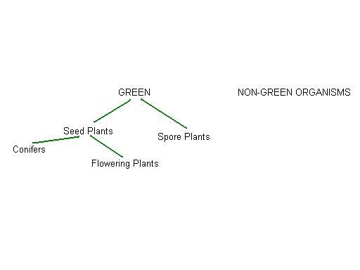

